Example Six: Non-linear Models

Our final example (file ExampleSix.RPF) is taken from Greene (2012), Section 7.2.5. This estimates a model of consumption of the form:

\begin{equation} C_t = \alpha + \beta Y_t^\gamma + \varepsilon _t \end{equation}

where \(C\) is (real) consumption, \(Y\) is (real) disposable personal income and \(\alpha\), \(\beta\) and \(\gamma\) are unknown parameters.

The data file is ExampleSix.RAT, which is a RATS data format file. If you open this (choose File—Open, pick “RATS Data Files” in the file type box, and select the file), you will see the following RATS Data File Window:

If you think that it looks a lot like a Series Window, you’re right. They are formatted the same way, and share most of the same operations on the View menu and toolbars.

Of the five series on the file, we need only two: REALCONS and REALDPI. Select those two (click on one of the series, then <Ctrl>+click or <Command>+click on the second), and choose the Data/Graphics—Data (RATS Format) menu operation. This will pop up the following dialog box:

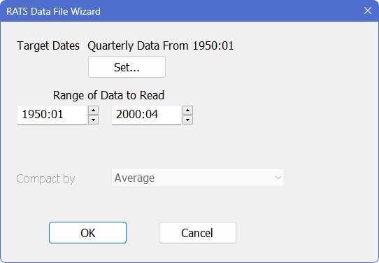
You’ll notice that this is much simpler than the Data Wizard for the other formats. What this wizard will do is to look at the series that you selected, and guess that you want the coarsest frequency and the maximum common range. For instance, if we had both monthly and quarterly data, with some series starting in 1947 and some in 1954, the guess would be quarterly data starting in 1954. If the common range is what you want, you can just OK the dialog. In this case, all the data are quarterly, and start and end at the same dates, so the only question is whether we want the whole range. If we wanted just 1960:1 to 1995:4, we could change the start and end dates in the dialog to request that range. We do want the full range, so we get

OPEN DATA "ExampleSix.rat"

CALENDAR(Q) 1950:1

DATA(FORMAT=RATS) 1950:01 2000:04 REALGDP REALCONS

If \(\gamma\) were known, we could create a transformed variable and estimate \(\alpha\) and \(\beta\) using LINREG; for instance, if it were 1.2, that would be done with:

set ypower = realdpi^1.2

linreg realcons

# constant ypower

Since it’s unknown, we can’t, and have to estimate this using the instruction NLLS (Non-Linear Least Squares).

Estimating linear models with least squares and related techniques is a fairly simple process, involving straightforward matrix computations. Non-linear estimation, however, is an inherently more general and complex task—the variety of different models you can estimate is virtually limitless, and fitting these models requires the application of complex iterative optimization algorithms, rather than simple computations.

The estimation process can demand a fair bit of expertise and judgment on the part of the user, because the algorithms can be sensitive to initial conditions and are prone to converging to local, rather than global, optima. Thus, it should be no surprise that fitting non-linear models in RATS requires more effort and attention than fitting simple OLS models.

There are several steps we must do before we can even estimate the model. First off, we need to decide what we will call the free parameters; we can’t use actual Greek characters, but we have to choose instead some legal RATS variable names.

Some other programs force you to use a specific way of writing this (perhaps c(1)+c(2)*realdpi^c(3)). RATS allows you to use symbolic names, which is much simpler, particularly if you ever decide to change the formula and add or remove some of the parameters. alpha, beta and gamma are an obvious choice here, but we’ll choose the shorter a, b and g. If we were doing a SET instruction to calculate the right-hand side formula, we could write that as a+b*realdpi^g, which is, in fact, the way that we will write this.

We need two instructions to tell RATS what the free parameters will be called and to define the right-hand side formula. These, respectively, are NONLIN and FRML. You might find it easiest to put these in manually, but you can also apply the Statistics—Equation/FRML Definition Wizard.

Equation/FRML Definition Wizard

Choose “FRML (General)” from the “Create” popup menu. Choose the name that you want to assign to this formula in the “Equation/FRML Name” box; we’ll use CFRML. Choose the dependent variable (REALCONS) in the “Dependent Variable” popup. Put in the names A B G in the “Free Parameters” box and the formula A+B*REALDPI^G in the “Formula” box. As you can see, since you have to type in both the formula and the parameter names, there isn’t all that much that the wizard really does other than help you make sure you get all the information in. For instance, if you just put in the formula definition without providing the A B G names, you will get an error message that A is unrecognizable when you try to OK the dialog.

If you put everything in correctly, the wizard will produce:

NONLIN a b g

FRML CFRML REALCONS = a+b*realdpi^g

The NONLIN instruction tells RATS that on non-linear estimation instructions that follow, the free parameters will be A, B and G. The FRML instruction (FRML short for FoRMuLa) defines the expression that we’ll be using—CFRML will be a special data type also known as a FRML. You don’t need to include the dependent variable when defining a FRML; if you don’t have one, just leave that part of the instruction out.

Guess Values

However, we’re still not quite ready. (As we said, non-linear estimation is quite a bit harder than linear). Non-linear least squares is an iterative process; Greene, in fact, shows how to do (roughly) what RATS will do internally as a whole sequence of linear regressions. That sequence has to start somewhere, at what are known as the guess values or initial values. The default for RATS is all zeros, which sometimes works fine. Zeros won’t work here, because if B is zero, the value of G doesn’t matter: G is said to be unidentified (more than one value for G, here all values, give the same result).

An obvious choice to start are least squares results when G is one, which would just be a LINREG of REALCONS on CONSTANT and REALDPI. We can set this up with

linreg realcons

# constant realdpi

compute a=%beta(1),b=%beta(2),g=1.0

%BETA is a vector defined by RATS which has the coefficients from the last estimation instruction. %BETA(1) is the first coefficient and %BETA(2) is the second. We use those in a COMPUTE instruction to put our guess values into the three parameters.

The NLLS Instruction

Finally, we’re ready. The model is estimated with

nlls(frml=cfrml)

Because of all the work required to prepare everything, the instruction itself is quite simple. NLLS has quite a few options, but most of them are to control the estimation process itself if the model proves hard to fit. The output is shown here:

Nonlinear Least Squares - Estimation by Gauss-Newton

Convergence in 65 Iterations. Final criterion was 0.0000003 <= 0.0000100

Dependent Variable REALCONS

Quarterly Data From 1950:01 To 2000:04

Usable Observations 204

Degrees of Freedom 201

Centered R^2 0.9988339

R-Bar^2 0.9988223

Uncentered R^2 0.9997776

Mean of Dependent Variable 2999.4357843

Std Error of Dependent Variable 1459.7066917

Standard Error of Estimate 50.0945979

Sum of Squared Residuals 504403.21571

Regression F(2,201) 86081.2782

Significance Level of F 0.0000000

Log Likelihood -1086.3906

Durbin-Watson Statistic 0.2960

Variable Coeff Std Error T-Stat Signif

********************************************************************************

1. A 458.79905447 22.50138682 20.38981 0.00000000

2. B 0.10085209 0.01091037 9.24369 0.00000000

3. G 1.24482749 0.01205479 103.26415 0.00000000

It’s not that much different from LINREG output. The only addition is the line describing the number of iterations. You would like this to indicate that the estimation has converged. If it doesn’t, you will see in its place something like:

NO CONVERGENCE IN 30 ITERATIONS

LAST CRITERION WAS 0.0273883

When you get this message, or something like it, pay attention; it’s telling you that something seems to be wrong. We get quite a few technical support questions where people are trying to interpret results (the bottom part of the output) while ignoring the message that the estimates might be wrong. This turns out to be a simple one to correct; we generated the warning message above by adding to NLLS the option ITERS=30 (which is less than the default of 100 iterations). Just taking off the restricted number of iterations (by omitting the ITERS option) gives us the proper result. In many cases, though, you have quite a bit more work to do to correct the reported problem. If you do non-linear estimation, you need to read (carefully) through the first few sections in "Non-linear Optimization".

Fitted Values

We introduced the PRJ instruction for computing fitted values in Example Five. PRJ also works for many other types of estimations. However, it doesn’t work after NLLS, or other instructions that aren’t based upon a linear specification. Instead, you can apply your defined FRML in a SET instruction:

set fitted = cfrml

A FRML can be used within the SET expression (or, for that matter, in another FRML definition) almost exactly like a series, that is, CFRML by itself means the value at the current entry, CFRML{1} means the value the previous entry, etc. However, these types of expressions are the only places where you can use a FRML like a series. You can’t use them for the dependent variable in a regression, or in the regressor list, or many other places. If you want to see the value produced by a FRML, do a SET as shown, and then examine the series created.

Learn More: Non-Linear Estimation Instructions

Many of the most important (and complicated) instructions in RATS do non-linear estimation. See Chapter 4 of the User’s Guide on non-linear estimation techniques, which describes the various optimization algorithms, methods of creating and maintaining non-linear parameter sets and formulas, and includes descriptions of several of the basic instructions.

The following are similar to NLLS in that they require a NONLIN instruction and one (or more) FRML’s to be defined before you can use them.

MAXIMIZE does maximum-likelihood estimation, applicable to a very large variety of models.

NLSYSTEM estimates systems of non-linear equations, rather than just the one equation that NLLS handles.

Most of the remaining instructions have sizable sections devoted to their use.

GARCH estimates univariate and multivariate ARCH and GARCH models.

DLM estimates and analyzes state-space models.

CVMODEL estimates covariance matrix models for structural VAR’s.

NPREG estimates non-parametric regressions.

LQPROG solves linear and quadratic programming problems.

NNLEARN and NNTEST fit neural networks.

FIND can be used for just about any other type of optimization problem. If the function to be optimized can be written out using RATS instructions, FIND can be used to optimize it.

Learn More: Working with Matrices

Matrices (or arrays—we use the terms interchangeably) are very useful in RATS. For example, above we showed how to use the %BETA vector to access estimated coefficients. %BETA is just one of many arrays defined by various RATS instructions. For example, LINREG and many others also save the estimated standard errors and t-statistics in the vectors %STDERRS and %TSTATS, respectively. Arrays like these can be useful in reporting results, and for doing further computations, such as the Hausman test.

DISPLAY and COMPUTE

By now you should be familiar with DISPLAY and COMPUTE, and won’t be surprised to learn they work with arrays as well as scalars. For example, after doing the NLLS instruction in our example, you could (re) display the estimated coefficients and standard errors (with fewer decimals) by doing:

?*.### %beta

?*.### %stderrs

COMPUTE is the primary instruction for doing matrix computations. RATS supports the standard arithmetic operators as well as several special matrix-specific operators. The program also provides dozens of built-in functions (such as inverse, transpose, and so on) for doing matrix calculations. See "Matrix Expressions" for more.

Defining Arrays

You can use DECLARE to create your own arrays, although you can often skip the declaration step. COMPUTE, READ, or INPUT can store values into arrays. If you need to construct an array from a set of series, you can do that using the MAKE instruction.

Other Types of Matrices

You can define arrays of labels, strings, series, equations, even arrays of arrays, and so on. These structures can be very useful in writing more sophisticated code, particularly for implementing complex, repetitive tasks. In "Graphics" we make extensive use of arrays of strings for labeling graphs, while instructions like FORECAST use arrays of series to store results.

In-Line Matrix Notation

You can use in-line matrix notation to provide the values of an array in an expression. Use two vertical lines (||) to mark the start and end of an array, and a single bar (|) for a row break. This is particularly useful for defining a matrix in the middle of an expression, such as in a non-linear formula. You can also use in-line matrix notation for options that accept an array for the arguments. For example, this estimates a Box-Jenkins model with AR terms on lags 1, 4, and 12:

boxjenk(ar=||1,4,12||) y