VECMGARCH.RPF

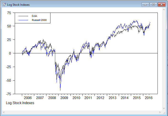
VECMGARCH.RPF is an example of some of the calculations done in Pardo and Torro(2007). This is applied to a different data set than in the paper; in this case, the closing weekly adjusted values for the Dow Jones Industrial Average and the Russell 2000 for the U.S. stock market. Note that, unlike most applications of GARCH to stock market data, these are not done in returns—if you convert to returns, you would lose the (possible) cointegration, and analyzing this as an error-correction GARCH model is the whole point. The two series are transformed to 100*log's and are normalized to both start at 0. The normalization has no effect on the model, but makes it easier to see (graphically) that the two series might be cointegrated.

set logdjia = 100.0*(log(djia/djia(1)))

set logrut = 100.0*(log(russell2000/russell2000(1)))

AIC and SBC (and HQ) pick very different lag lengths. The SBC picks 1, which seems too short. We use 4 in the subsequent analysis, which is a compromise which is at least a local minimum in the AIC. Note that the lag selection criteria assume homoscedasticity, and so can be thrown off by GARCH error processes.

There's no strong reason to believe that the two stock indexes are cointegrated since they have different risk-return structures. The Johansen test allowing for trending data is done with @JOHMLE. The Johansen test is known to be at least somewhat robust to a GARCH error process.

@johmle(lags=nlags,det=constant,cv=cv)

# logdjia logrut

The Johansen test marginally rejects cointegration, but we'll go ahead and assign cointegration rank one for illustrative purposes. This uses the estimated cointegrating vector. In other applications (for instance with spot vs futures prices), the cointegrating vector will be known theoretically, and you should use that, not an estimated one.

This sets up a VECM for the DET=CONSTANT model (including a CONSTANT as a DET term in the VAR). For this, you put in the original dependent variables, not the differences. The rearrangement of the regression is done internally when you ESTIMATE the model.

equation(coeffs=cv) ecteq *

# logdjia logrut

system(model=basevecm)

variables logdjia logrut

lags 1 to nlags

det constant

ect ecteq

end(system)

The error correction model is first estimated by least squares, and a test for ARCH is done on the residuals with @MVARCHTEST, which overwhelmingly rejects homoscedasticity.

estimate(resids=vecmresids)

@mvarchtest(lags=5)

# vecmresids

This estimates an asymmetric BEKK GARCH model. This saves the jointly standardized residuals (as STDU), the conditional covariance matrices (HH) and (non-standardized) residuals (RR) and the VECH representation (VECHCOMPS):

garch(model=basevecm,mv=bekk,asymmetric,stdresids=stdu,hmatrices=hh,rvectors=rr,$

pmethod=simplex,piters=10,method=bfgs,iters=500,vechmat=vechcomps)

One thing to note in the output is that neither of the error correction terms is significant. If the series were truly cointegrated (again, we are doing this as a VECM for illustration) at least one of these two should be significant. These t-statistics are the tests for long-run causality.

This does the recommended set of multivariate residual diagnostics (for remaining ARCH and for serial correlation in the mean):

@mvarchtest(lags=5)

# stdu

@mvqstat(lags=5)

# stdu

The results pass easily.

These next lines do causality tests in the mean. The first does a joint test for whether the dx2 lags and the ect lag are zero in the first equation (first block of mean model coefficients) and the second does a similar test for the dx1 lags and ect in the second block of mean model coefficients. The simplest way to set these up is to use the Regression Tests, Exclusion Restrictions test wizard. Note that the Pardo-Torro paper doesn't include the lagged ECT in the test, but it should be included since if it's non-zero, the lagged "other" does help to predict. The wizard dialog for the x2 to x1 causality will look something like

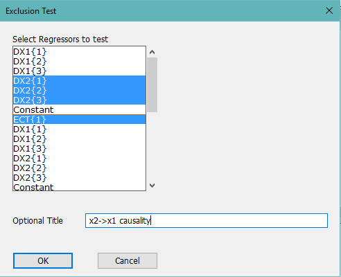
The first block of regressors is for the first equation, so this will do a joint test on the DX2 lags and the ECT lag for that.

test(zeros,title="x2-->x1 causality")

# 4 5 6 8

test(zeros,title="x1-->x2 causality")

# 9 10 11 16

Neither direction is significant. There are also tests on the BEKK cross effects (joint test of all the off-diagonal A, B and D coefficients) and a joint test on all the asymmetry (D) coefficients. Again, it's easiest to set these up using the Regression Tests wizard.

There are also diagnostics on the univariate standardized residuals:

set std1 = rr(t)(1)/sqrt(hh(t)(1,1))

set std2 = rr(t)(2)/sqrt(hh(t)(2,2))

You can only do univariate tests (not joint ones like @MVARCHTEST) on these. Again, these pass all the tests. However, note well that we chose to fit this under the assumption of cointegration despite the fact that the initial test showed that to be likely incorrect—the model is probably more complicated than it needs to be to adequately explain the data.

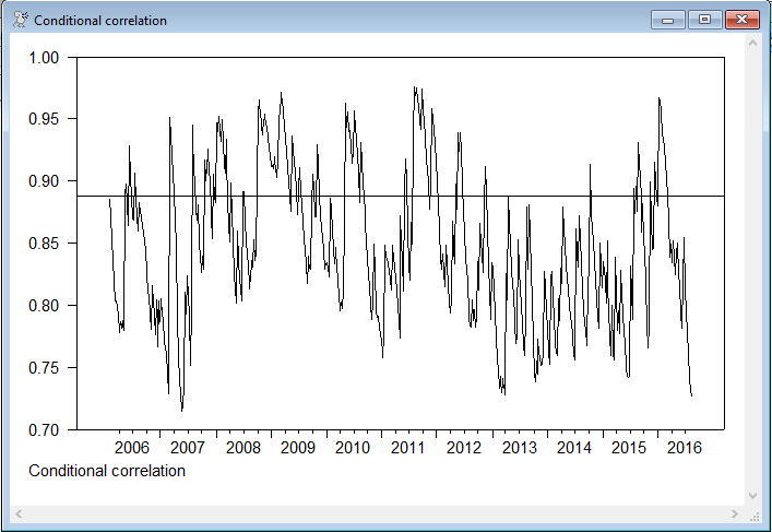
None of the remaining analysis has anything to do with this being a VECM-GARCH model—they're general to the multivariate GARCH model. Graphs are done of the conditional volatility (in standard deviations, which aren't dominated by the more extreme values as the variances), the conditional correlation and the conditional beta. All of these can be done (in pretty much the same way) for any type of multivariate GARCH model.

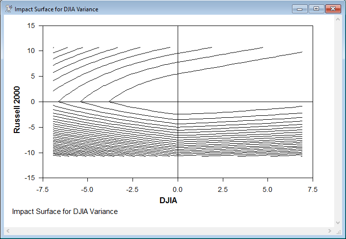
The final calculations are impact surfaces for the two variances and the covariance with respect to lagged residuals. This can be computed (easily) for any multivariate GARCH model which has a VECH representation (DVECH, VECH or any form of BEKK), but the graphs are specific to this being a two-variable model, since it does a contour graph with axes for each shock.

Full Program

open data "usstocks.xls"
calendar(w) 2006:1:2
*
* The data were taken from Yahoo Finance and are in reversed
* chronological order. RATS v9.1 automatically detects that and
* rearranges the data. (The REVERSE option has no effect, but creates an
* immediate error with earlier versions of RATS).
*
data(format=xls,org=columns,reverse) / djia russell2000
*
* Normalize both to 100 * log relative to the first entry
*
set logdjia = 100.0*(log(djia/djia(1)))
set logrut = 100.0*(log(russell2000/russell2000(1)))
*
graph(footer="Log Stock Indexes",key=upleft,klabels=||"DJIA","Russell 2000"||) 2
# logdjia
# logrut
*
* AIC and SBC (or HQ) pick very different lag lengths. The 1 favored by
* SBC and HQ seems too short. AIC has a local minimum at 4, so we choose
* that. (None of these criteria are designed for heteroscedastic data,
* so they can be thrown off by outliers).
*
@varlagselect(lags=10,crit=aic)
# logdjia logrut
@varlagselect(lags=10,crit=sbc)
# logdjia logrut
*
compute nlags=4
*
* There's no strong reason to believe that the two stock indexes are
* cointegrated since they have different risk-return structures. The
* Johansen test marginally rejects cointegration, but we'll go ahead and
* assign cointegration rank one for illustrative purposes. This uses the
* estimated cointegrating vector. In other applications (for instance
* with spot vs futures prices), the cointegrating vector will be known
* theoretically, and you should use that, not an estimated one.
*
* This analyzes cointegration using DET=CONSTANT, which allows for a
* trend in the series.
*
@johmle(lags=nlags,det=constant,cv=cv)
# logdjia logrut
*
* This sets up a VECM for the DET=CONSTANT model (including a CONSTANT
* as a DET term in the VAR). For this, you put in the original dependent
* variables, not the differences. The rearrangement of the regression is
* done internally when you ESTIMATE the model.
*
equation(coeffs=cv) ecteq *
# logdjia logrut
*
system(model=basevecm)
variables logdjia logrut
lags 1 to nlags
det constant
ect ecteq
end(system)
*
estimate(resids=vecmresids)
*
* Note that the number of lags used in the diagnostic tests has nothing
* to do with the choice of the number of lags in the VAR model. (The
* paper does some tests later on the OLS VECM residuals and uses 5 for
* those). Somewhere in the 3-5 lag range generally seems appropriate for
* this.
*
@mvarchtest(lags=5)
# vecmresids
*
* Estimate an asymmetric BEKK GARCH model. This saves the jointly
* standardized residuals (as STDU), the conditional covariance matrices
* (HH) and (non-standardized) residuals (RR) and the VECH representation
* (VECHCOMPS).
*
garch(model=basevecm,mv=bekk,asymmetric,stdresids=stdu,hmatrices=hh,rvectors=rr,$
pmethod=simplex,piters=10,method=bfgs,iters=500,vechmat=vechcomps)
*
* These are (our) recommended diagnostic tests on the jointly standardized
* residuals. Tests on the univariate standardized residuals come later.
*
@mvarchtest(lags=5)
# stdu
@mvqstat(lags=5)
# stdu
*
* Causality tests in the mean. The first tests does a joint test for
* whether the dx2 lags and the ect lag are zero in the first equation
* (first block of mean model coefficients) and the second does a similar
* test for the dx1 lags and ect in the second block of mean model
* coefficients. (You can use the Statistics-Regression Tests, Exclusion
* Restrictions wizard to set these up.)
*
* (The paper doesn't include the ECT in the test, but it should be
* included since if it's non-zero, the lagged "other" does help to
* predict).
*
test(zeros,title="x2-->x1 causality")
# 4 5 6 8
test(zeros,title="x1-->x2 causality")
# 9 10 11 16
*
* Wald tests of BEKK coefficients
*
test(zeros,title="BEKK cross effects")
# 21 22 25 26 29 30
test(zeros,title="Asymmetry")
# 28 29 30 31
*
* Tests on the univariate standardized residuals
*
set std1 = rr(t)(1)/sqrt(hh(t)(1,1))
set std2 = rr(t)(2)/sqrt(hh(t)(2,2))
*
* Skewness, (excess) kurtosis and normality (Jarque-Bera) are all part
* of the standard STATISTICS output.
*
stats std1
stats std2
*
* The Q(20) (Ljung-Box) and Q^2(20) (McLeod-Li) are included in the
* BDINDTESTS procedure.
*
@bdindtests(number=20) std1
@bdindtests(number=20) std2
*
* You can also do the LB and McLeod-Li tests separately using @RegCorrs
* (for LB) and @McLeodLi. The results are very slightly different
* because they use a slightly different calculation for the
* autocorrelations.
*
@regcorrs(qstats,number=20) std1
@mcleodli(number=20) std1
@archtest(lags=20) std1
*
@regcorrs(qstats,number=20) std2
@mcleodli(number=20) std2
@archtest(lags=20) std2
*
* These graph the conditional volatility (in standard deviations to
* allow more detail to be seen), the conditional correlation and the
* conditional beta. The latter two also include a horizontal line at the
* corresponding value from the original VECM estimates.
*
set sig11 = sqrt(hh(t)(1,1))
set sig22 = sqrt(hh(t)(2,2))
graph(footer="Conditional Volatility in Std Deviations",$
   key=below,klabels=||"DJIA","Russell 2000"||) 2
# sig11
# sig22
*
set rho12 = %cvtocorr(hh(t))(1,2)
graph(footer="Conditional correlation",vgrid=%cvtocorr(%sigma)(1,2))
# rho12
*
set beta12 = hh(t)(1,2)/hh(t)(1,1)
graph(footer="Conditional beta of Russell 2000 with respect to DJIA",$
   vgrid=%sigma(1,2)/%sigma(1,1))
# beta12
*
* Compute impact surfaces (done as contour graphs)
*
compute ngrid=21
*
* This picks the grids in each direction based upon the observed
* absolute values of the residuals from the VECM (going from - to + of
* the 99%-ile of the absolute value).
*
set plus1 = abs(vecmresids(1))
stats(fract,noprint) plus1
compute grid1=%seqrange(-%fract99,+%fract99,ngrid)
set plus2 = abs(vecmresids(2))
stats(fract,noprint) plus2
compute grid2=%seqrange(-%fract99,+%fract99,ngrid)
*
dec rect var1g(ngrid,ngrid) var2g(ngrid,ngrid) covarg(ngrid,ngrid)
*
do i=1,ngrid
   do j=1,ngrid
      compute [symm] response=%vectosymm($
            vechcomps("A")*%vec(%outerxx(||grid1(i)|grid2(j)||))+$
            vechcomps("D")*%vec(%outerxx(||%minus(grid1(i))|%minus(grid2(j))||)),$
            2)
      compute var1g(i,j)=response(1,1)
      compute var2g(i,j)=response(2,2)
      compute covarg(i,j)=response(1,2)
   end do j
end do i
*
* Do contour plots
*
gcontour(x=grid1,y=grid2,f=var1g,hlabel="DJIA",vlabel="Russell 2000",$
footer="Impact Surface for DJIA Variance")
gcontour(x=grid1,y=grid2,f=var2g,hlabel="DJIA",vlabel="Russell 2000",$
footer="Impact Surface for Russell 2000 Variance")
gcontour(x=grid1,y=grid2,f=covarg,hlabel="DJIA",vlabel="Russell 2000",$
footer="Impact Surface for Covariance")

Output

VAR Lag Selection

Lags AICC

0 15.9792555

1 8.2352485

2 8.2361942

3 8.2354481

4 8.2272985

5 8.2287103

6 8.2358474

7 8.2135519*

8 8.2143388

9 8.2213291

10 8.2286912

VAR Lag Selection

Lags SBC/BIC

0 15.9915266

1 8.2720192*

2 8.2974074

3 8.3210460

4 8.3372231

5 8.3629029

6 8.3942490

7 8.3961029

8 8.4209793

9 8.4519985

10 8.4833285

Likelihood Based Analysis of Cointegration

Variables: LOGDJIA LOGRUT

Estimated from 2006:01:30 to 2020:08:10

Data Points 759 Lags 4 with Constant

Unrestricted eigenvalues, -T log(1-lambda) and Trace Test

Roots Rank EigVal Lambda-max Trace Trace-95%

2 0 0.0125 9.5275 10.3932 15.3400

1 1 0.0011 0.8657 0.8657 3.8400

Cointegrating Vector for Largest Eigenvalue

LOGDJIA LOGRUT

-0.168654 0.130579

VAR/System - Estimation by Cointegrated Least Squares

Weekly Data From 2006:01:30 To 2020:08:10

Usable Observations 759

Dependent Variable LOGDJIA

Mean of Dependent Variable 0.0828052299

Std Error of Dependent Variable 2.3021718535

Standard Error of Estimate 2.2865403259

Sum of Squared Residuals 3926.4282631

Durbin-Watson Statistic 2.0046

Variable Coeff Std Error T-Stat Signif

************************************************************************************

1. D_LOGDJIA{1} -0.049703854 0.071699459 -0.69322 0.48838272

2. D_LOGDJIA{2} 0.119169085 0.071973693 1.65573 0.09819403

3. D_LOGDJIA{3} -0.061265243 0.071875202 -0.85238 0.39427297

4. D_LOGRUT{1} 0.013719874 0.053791745 0.25506 0.79875015

5. D_LOGRUT{2} -0.059179461 0.053736351 -1.10129 0.27112204

6. D_LOGRUT{3} -0.049054788 0.053545600 -0.91613 0.35989224

7. Constant -0.070703634 0.190250917 -0.37163 0.71027049

8. EC1{1} 0.079487651 0.082996156 0.95773 0.33850870

Dependent Variable LOGRUT

Mean of Dependent Variable 0.1237170066

Std Error of Dependent Variable 3.0781015253

Standard Error of Estimate 3.0650010017

Sum of Squared Residuals 7055.0675865

Durbin-Watson Statistic 1.9957

Variable Coeff Std Error T-Stat Signif

************************************************************************************

1. D_LOGDJIA{1} 0.068398090 0.096109791 0.71167 0.47689250

2. D_LOGDJIA{2} 0.233982630 0.096477389 2.42526 0.01553225

3. D_LOGDJIA{3} -0.086128520 0.096345367 -0.89396 0.37163181

4. D_LOGRUT{1} -0.060815734 0.072105334 -0.84343 0.39925708

5. D_LOGRUT{2} -0.115187050 0.072031080 -1.59913 0.11021235

6. D_LOGRUT{3} -0.014199461 0.071775388 -0.19783 0.84323013

7. Constant 0.278516870 0.255022510 1.09213 0.27512768

8. EC1{1} -0.072420206 0.111252488 -0.65095 0.51527557

Multivariate ARCH Test

Statistic Degrees Signif

473.79 45 0.00000

MV-GARCH, BEKK - Estimation by BFGS

Convergence in 134 Iterations. Final criterion was 0.0000000 <= 0.0000100

Weekly Data From 2006:01:30 To 2020:08:10

Usable Observations 759

Log Likelihood -2941.5485

Variable Coeff Std Error T-Stat Signif

************************************************************************************

Mean Model(LOGDJIA)

1. D_LOGDJIA{1} -0.043763647 0.060086512 -0.72834 0.46640306

2. D_LOGDJIA{2} 0.036723159 0.056000685 0.65576 0.51197683

3. D_LOGDJIA{3} -0.093426788 0.055747981 -1.67588 0.09376219

4. D_LOGRUT{1} 0.011370267 0.042423556 0.26802 0.78868564

5. D_LOGRUT{2} -0.034424126 0.041568156 -0.82814 0.40759294

6. D_LOGRUT{3} 0.039632920 0.042197520 0.93922 0.34761580

7. Constant -0.075739179 0.147442108 -0.51369 0.60747044

8. EC1{1} 0.083814979 0.060300642 1.38995 0.16454355

Mean Model(LOGRUT)

9. D_LOGDJIA{1} 0.028377503 0.081875208 0.34659 0.72889592

10. D_LOGDJIA{2} 0.087792063 0.077602752 1.13130 0.25792847

11. D_LOGDJIA{3} -0.068980642 0.078063419 -0.88365 0.37688586

12. D_LOGRUT{1} -0.043920165 0.060368653 -0.72753 0.46689973

13. D_LOGRUT{2} -0.063394688 0.059101909 -1.07263 0.28343558

14. D_LOGRUT{3} 0.027708083 0.059374618 0.46667 0.64073926

15. Constant 0.196340052 0.195734076 1.00310 0.31581459

16. EC1{1} -0.024338175 0.081203598 -0.29972 0.76439232

17. C(1,1) 0.536742145 0.087928428 6.10431 0.00000000

18. C(2,1) 1.011704111 0.133694310 7.56729 0.00000000

19. C(2,2) 0.001824514 0.134337611 0.01358 0.98916382

20. A(1,1) -0.088499362 0.130987858 -0.67563 0.49927542

21. A(1,2) -0.449294604 0.167375786 -2.68435 0.00726717

22. A(2,1) 0.107685498 0.100836352 1.06792 0.28555507

23. A(2,2) 0.356808843 0.132576854 2.69134 0.00711665

24. B(1,1) 1.053401968 0.032624545 32.28863 0.00000000

25. B(1,2) 0.150456003 0.056120300 2.68096 0.00734124

26. B(2,1) -0.155429493 0.033309666 -4.66620 0.00000307

27. B(2,2) 0.746215374 0.054142386 13.78246 0.00000000

28. D(1,1) 0.132160274 0.099141459 1.33305 0.18251622

29. D(1,2) 0.002417575 0.153900038 0.01571 0.98746676

30. D(2,1) 0.311238147 0.070389598 4.42165 0.00000980

31. D(2,2) 0.498929282 0.116488548 4.28308 0.00001843

Multivariate ARCH Test

Statistic Degrees Signif

47.81 45 0.35941

Multivariate Q Test

Test Run Over 2006:01:30 to 2020:08:10

Lags Tested 5

Degrees of Freedom 20

Q Statistic 11.06726

Signif Level 0.94446

x2-->x1 causality

Chi-Squared(4)= 3.961522 or F(4,*)= 0.99038 with Significance Level 0.41123831

x1-->x2 causality

Chi-Squared(4)= 2.229419 or F(4,*)= 0.55735 with Significance Level 0.69364712

BEKK cross effects

Chi-Squared(6)= 58.532676 or F(6,*)= 9.75545 with Significance Level 0.00000000

Asymmetry

Chi-Squared(4)= 87.878354 or F(4,*)= 21.96959 with Significance Level 0.00000000

Statistics on Series STD1

Weekly Data From 2006:01:30 To 2020:08:10

Observations 759

Sample Mean -0.002279 Variance 0.994189

Standard Error 0.997090 SE of Sample Mean 0.036192

t-Statistic (Mean=0) -0.062965 Signif Level (Mean=0) 0.949811

Skewness -0.520557 Signif Level (Sk=0) 0.000000

Kurtosis (excess) 0.667615 Signif Level (Ku=0) 0.000186

Jarque-Bera 48.374556 Signif Level (JB=0) 0.000000

Statistics on Series STD2

Weekly Data From 2006:01:30 To 2020:08:10

Observations 759

Sample Mean 0.003256 Variance 0.986803

Standard Error 0.993380 SE of Sample Mean 0.036057

t-Statistic (Mean=0) 0.090308 Signif Level (Mean=0) 0.928066

Skewness -0.462865 Signif Level (Sk=0) 0.000000

Kurtosis (excess) 0.344532 Signif Level (Ku=0) 0.053782

Jarque-Bera 30.855813 Signif Level (JB=0) 0.000000

Independence Tests for Series STD1

Test Statistic P-Value

Ljung-Box Q(20) 17.218262 0.6388

McLeod-Li(20) 18.178192 0.5757

Turning Points 1.924922 0.0542

Difference Sign -1.507874 0.1316

Rank Test 0.377956 0.7055

Independence Tests for Series STD2

Test Statistic P-Value

Ljung-Box Q(20) 10.5891603 0.9562

McLeod-Li(20) 14.1788376 0.8213

Turning Points 0.5458733 0.5852

Difference Sign 0.3769685 0.7062

Rank Test 0.2374944 0.8123

McLeod-Li Test for Series STD1

Using 759 Observations from 2006:01:30 to 2020:08:10

Test Stat Signif

McLeod-Li(20-0) 17.8764915 0.59554

Test for ARCH in STD1

Using data from 2006:01:30 to 2020:08:10

Lags Statistic Signif. Level

20 0.870 0.62672

McLeod-Li Test for Series STD2

Using 759 Observations from 2006:01:30 to 2020:08:10

Test Stat Signif

McLeod-Li(20-0) 14.0530485 0.82780

Test for ARCH in STD2

Using data from 2006:01:30 to 2020:08:10

Lags Statistic Signif. Level

20 0.697 0.83174

Graphs

This is a graph of the normalized log data

Graph of the conditional correlation with the correlation of the fixed VECM residuals shown.

One of the news impact surfaces, graphed as a contour graph for the impact versus the shocks in the two variables. Even though this is for the variance of the DJIA, it is most heavily impacted by the negative lagged shocks in the Russell 2000 (the contours are steepest in the negative Y direction).