Gray JFE 1996 Markov Switching GARCH model

[jack]

I use this code (a part of the code):

Code: Select all

*
*
* Regime-switching GARCH
*
nonlin a01 a02 a11 a12 b01 b11 b21 b02 b12 b22 p
compute a01=%beta(1),a11=%beta(2),b01=olsvar,b11=0.0,b21=0.0
compute a02=%beta(1),a12=%beta(2),b02=%beta(3),b12=%beta(4),b22=%beta(5)
compute p=||.95,.05||
*
set uu = olsvar
set h  = olsvar
*
* RegimeGARCHF returns the 2 vector of densities in the two regimes.
* Again, many lines in this are specific to the problem at hand.
*
function RegimeGARCHF t
type vector RegimeGARCHF
type integer t
local real hh1 hh2 mu1 mu2 mu
*
* Compute state dependent variances
*
compute hh1=b01+b11*uu(t-1)+b21*h(t-1)
compute hh2=b02+b12*uu(t-1)+b22*h(t-1)
*
* Compute state dependent means
*
compute mu1=a01+a11*rate(t-1)
compute mu2=a02+a12*rate(t-1)
*
* Compute the return vector (densities in the two states)
*
compute RegimeGARCHF=||%density((drate(t)-mu1)/sqrt(hh1))/sqrt(hh1),$
                       %density((drate(t)-mu2)/sqrt(hh2))/sqrt(hh2)||
*
* Compute the values of uu (squared residual) and h (variance) to be
* used for the period following.
*
compute mu=mu1*pstar(1)+mu2*pstar(2)
compute uu(t)=(drate(t)-mu)^2
compute h(t)=pstar(1)*(mu1^2+hh1)+pstar(2)*(mu2^2+hh2)-mu^2
end
*
frml logl = f=RegimeGARCHF(t),fpt=%MSProb(t,f),log(fpt)
*
* This combination is able to locate Gray's results - the first MAXIMIZE
* works with the "p" matrix fixed at a fairly high level of persistence,
* and tries to get estimates which separate the two states. The second
* then adds the p matrix to the parmset.
*
nonlin a01 a02 a11 a12 b01 b11 b21 b02 b12 b22
maximize(start=(pstar=%MSInit()),method=bfgs,iters=100,pmethod=simplex,piters=50) logl 2 *
nonlin a01 a02 a11 a12 b01 b11 b21 b02 b12 b22 p
maximize(start=(pstar=%MSInit()),method=bfgs,iters=100) logl 2 *
*
* Compute the smoothed probabilities and the ex ante probabilities
*
@MSSmoothed %regstart() %regend() psmooth
set exante %regstart() %regend() = pt_t1(t)(1)
set smooth %regstart() %regend() = psmooth(t)(1)
*
* And the conditional standard deviation
*
set condstddev = sqrt(exante*b01^2+(1-exante)*b02^2)
*
spgraph(vfields=2,window="Figure 5")
graph(max=1.0,header="Regime Probabilities") 2
# exante
# smooth
graph(header="Conditional Standard Deviation")
# condstddev
spgraph(done)

I did the calculations after the MAXIMIZE instruction for the MS-GARCH. But I'm not sure if I'm doing the right thing about H.

[TomDoan]

That's just repeating the values from the previous model. The MS-GARCH computes H as the ex-ante variance, and that's what you need:

set condstddev = sqrt(h)

[jack]

I really appreciate your kind replies and I'm so sorry for asking so many questions.
Here is the graph.
I would be grateful if I could possibly have your final word about it. Doesn't it mimic probabilities again?

figure 5.png (17.71 KiB) Viewed 45452 times

[TomDoan]

First of all, isn't that effectively the same graph as in the paper? But no, compare the 1980-1982 range. The probabilities are relatively flat and the standard deviations are very spiky. If you compare the graph with the switching by non-GARCH variances, where the probabilities are flat, so are the standard deviations.

[jack]

Dear Tom,
I searched for smoothed and ex ante probabilities and studied Gray's paper about it. Unfortunately, I didn't find a satisfactory answer for it. To be clear, I don't know what's the difference between them intuitively? Which one is more important?

[TomDoan]

I'm not sure there's any "intuition" involved. The ex ante probability at t uses only the observations before t. It's used in computing the likelihood and any diagnostics. The smoothed probability is the probability using all the data (before, during and after). If you consider, for instance, Hamilton's model of GDP growth, the smoothed probability of recession would be the best to compare with NBER definitions, since the NBER decides when recessions begin and end several quarters later and thus use future data as well.

[jack]

Dear Tom,
Is it posssible to test the statistical significance of the second regime When comparing the regime-switching
GARCH model with the single-regime GARCH model? In the Gray's paper it has been said that The quasi- LRT can no longer be assumed to be distributed as a chi-squared but in this paper http://onlinelibrary.wiley.com/doi/10.1 ... 3/abstract it has been said that "it is common practice to approximate the critical values of these conventional LR tests by the quantiles of the chi-squared distribution with degrees of freedom equal to the difference in the number of parameters between the two-regimes (alternative) and the single-regime specification (null hypothesis)".
Is it possible finally to use LRT to test the number of Markov regimes?

[TomDoan]

Sometimes "common practice" is not technically correct and this is one of those cases. I assume the idea is that if the restricted model is overwhelmingly rejected vs the MS model, then the fact that the LRT isn't really chi-squared asymptotically isn't all that important. This thread is about a calculation of a conservative bound on the LRT in situations like this, but one thing to note is that the MS-GARCH model doesn't compute the actual log likelihood of the model, but only an approximation. I don't know if it's clear whether the approximation understates or overstates the true LL of the model.

[jack]

Dear Tom,
I estimated a model using Gray's code. Here is the results. Is there enough evidence about the existence of second regime?
I don't know why P(1,2) is such low. What does is mean here? Especially, why is A12 greater than minus one? Does it has show that something is wrong with the model?

Linear Regression - Estimation by Least Squares
With Heteroscedasticity-Consistent (Eicker-White) Standard Errors
Dependent Variable DRATE
Daily(5) Data From 2003:01:06 To 2012:12:06
Usable Observations                      2589
Degrees of Freedom                       2587
Centered R^2                        0.2162382
R-Bar^2                             0.2159353
Uncentered R^2                      0.2162382
Mean of Dependent Variable       -0.000019215
Std Error of Dependent Variable   0.710001062
Standard Error of Estimate        0.628687695
Sum of Squared Residuals         1022.5071405
Log Likelihood                     -2471.0231
Durbin-Watson Statistic                2.3494

    Variable                        Coeff      Std Error      T-Stat      Signif
************************************************************************************
1.  Constant                      0.000001372  0.012350981 1.11101e-004  0.99991135
2.  DRATE{1}                     -0.465022692  0.029848275    -15.57955  0.00000000


MAXIMIZE - Estimation by BFGS
Convergence in    14 Iterations. Final criterion was  0.0000048 <=  0.0000100
Daily(5) Data From 2003:01:03 To 2012:12:06
Usable Observations                      2590
Function Value                     -1233.4961

    Variable                        Coeff      Std Error      T-Stat      Signif
************************************************************************************
1.  A01                           0.034373643  0.016306202      2.10801  0.03503009
2.  A02                          -0.018158900  0.005627435     -3.22685  0.00125160
3.  A11                          -0.987049117  0.024645457    -40.04994  0.00000000
4.  A12                          -1.036718008  0.031279355    -33.14384  0.00000000
5.  B01                           0.676242638  0.013864548     48.77495  0.00000000
6.  B02                           0.178090890  0.005701714     31.23462  0.00000000
7.  P(1,1)                        0.964435993  0.006934697    139.07400  0.00000000
8.  P(1,2)                        0.038301809  0.005753795      6.65679  0.00000000

Lag  Corr  Partial   LB Q    Q Signif
  1  0.089   0.089  20.64769    0.0000
  2  0.309   0.303 268.42934    0.0000
  3  0.122   0.084 307.28896    0.0000
  4  0.101  -0.003 333.89765    0.0000
  5  0.082   0.018 351.45483    0.0000
  6  0.031  -0.013 354.02735    0.0000
  7  0.044   0.006 359.06825    0.0000
  8  0.022   0.006 360.29757    0.0000
  9  0.055   0.041 368.24714    0.0000
 10  0.052   0.040 375.21940    0.0000
 11  0.068   0.039 387.30424    0.0000
 12  0.089   0.056 408.03453    0.0000
 13  0.072   0.028 421.61656    0.0000
 14  0.111   0.057 453.70138    0.0000
 15  0.091   0.043 475.14533    0.0000


GARCH Model - Estimation by BFGS
Convergence in    31 Iterations. Final criterion was  0.0000059 <=  0.0000100
Dependent Variable DRATE
Daily(5) Data From 2003:01:06 To 2012:12:06
Usable Observations                      2589
Log Likelihood                     -1640.8258

    Variable                        Coeff      Std Error      T-Stat      Signif
************************************************************************************
1.  Constant                     -0.002580050  0.004870402     -0.52974  0.59629165
2.  DRATE{1}                     -0.486710196  0.017265759    -28.18933  0.00000000

3.  C                             0.001934000  0.000469922      4.11558  0.00003862
4.  A                             0.318002213  0.026901340     11.82105  0.00000000
5.  B                             0.744130400  0.017127159     43.44739  0.00000000

Lag  Corr  Partial   LB Q    Q Signif
  1 -0.031  -0.031  2.552248    0.1101
  2  0.070   0.069 15.294223    0.0005
  3 -0.028  -0.024 17.282169    0.0006
  4 -0.015  -0.021 17.855229    0.0013
  5 -0.039  -0.037 21.893056    0.0005
  6 -0.043  -0.043 26.625084    0.0002
  7 -0.036  -0.035 30.074676    0.0001
  8 -0.038  -0.037 33.871933    0.0000
  9 -0.032  -0.034 36.612003    0.0000
 10 -0.001  -0.003 36.617247    0.0001
 11 -0.022  -0.025 37.857947    0.0001
 12 -0.011  -0.021 38.194854    0.0001
 13 -0.012  -0.017 38.548140    0.0002
 14 -0.029  -0.037 40.769661    0.0002
 15  0.002  -0.006 40.779242    0.0003


MAXIMIZE - Estimation by BFGS
Convergence in     9 Iterations. Final criterion was  0.0000091 <=  0.0000100
Daily(5) Data From 2003:01:03 To 2012:12:06
Usable Observations                      2590
Function Value                     -1054.8672

    Variable                        Coeff      Std Error      T-Stat      Signif
************************************************************************************
1.  A01                           0.013619894  0.013106682      1.03916  0.29873196
2.  A02                          -0.014933917  0.004393704     -3.39894  0.00067649
3.  A11                          -0.935668475  0.028987754    -32.27806  0.00000000
4.  A12                          -1.064079366  0.034639104    -30.71902  0.00000000
5.  B01                           0.067855137  0.006098469     11.12659  0.00000000
6.  B11                           0.136280582  0.028697956      4.74879  0.00000205
7.  B21                           0.807379310  0.029557752     27.31532  0.00000000
8.  B02                           0.003801359  0.000683465      5.56189  0.00000003
9.  B12                           0.310732981  0.049463576      6.28206  0.00000000
10. B22                           0.292483566  0.028278038     10.34313  0.00000000


MAXIMIZE - Estimation by BFGS
Convergence in    21 Iterations. Final criterion was  0.0000094 <=  0.0000100
Daily(5) Data From 2003:01:03 To 2012:12:06
Usable Observations                      2590
Function Value                     -1050.5437

    Variable                        Coeff      Std Error      T-Stat      Signif
************************************************************************************
1.  A01                           0.010285521  0.012745732      0.80698  0.41967938
2.  A02                          -0.015746220  0.004411478     -3.56937  0.00035783
3.  A11                          -0.934642290  0.030346397    -30.79912  0.00000000
4.  A12                          -1.085577499  0.037463795    -28.97671  0.00000000
5.  B01                           0.050692332  0.009910202      5.11517  0.00000031
6.  B11                           0.157356240  0.031981527      4.92022  0.00000086
7.  B21                           0.802614140  0.049317631     16.27439  0.00000000
8.  B02                           0.003374801  0.001166368      2.89343  0.00381063
9.  B12                           0.229441167  0.070668669      3.24672  0.00116744
10. B22                           0.246944292  0.038749720      6.37280  0.00000000
11. P(1,1)                        0.960576407  0.013708449     70.07185  0.00000000
12. P(1,2)                        0.075710440  0.020554312      3.68343  0.00023011


MAXIMIZE - Estimation by BFGS
NO CONVERGENCE IN 12 ITERATIONS
LAST CRITERION WAS  0.0000000
SUBITERATIONS LIMIT EXCEEDED.
ESTIMATION POSSIBLY HAS STALLED OR MACHINE ROUNDOFF IS MAKING FURTHER PROGRESS DIFFICULT
TRY HIGHER SUBITERATIONS LIMIT, TIGHTER CVCRIT, DIFFERENT SETTING FOR EXACTLINE OR ALPHA ON NLPAR
RESTARTING ESTIMATION FROM LAST ESTIMATES OR DIFFERENT INITIAL GUESSES MIGHT ALSO WORK
Daily(5) Data From 2003:01:03 To 2012:12:06
Usable Observations                      2590
Function Value                     -1018.0690

    Variable                        Coeff      Std Error      T-Stat      Signif
************************************************************************************
1.  A01                          -0.013393998  0.000380707    -35.18194  0.00000000
2.  A02                           0.045332574  0.002076028     21.83620  0.00000000
3.  A11                          -1.097700039  0.005548809   -197.82625  0.00000000
4.  A12                          -0.303118795  0.027167144    -11.15755  0.00000000
5.  B01                          -0.001011178  0.000002767   -365.49626  0.00000000
6.  B11                           0.059900700  0.000807929     74.14101  0.00000000
7.  B21                           0.609069171  0.000384612   1583.59479  0.00000000
8.  B02                           0.019938741  0.000145776    136.77666  0.00000000
9.  B12                           0.045280994  0.000174983    258.77336  0.00000000
10. B22                           1.870801841  0.029521412     63.37101  0.00000000
11. P(1,1)                        0.820696725  0.000355251   2310.18726  0.00000000
12. P(1,2)                        0.723588475  0.006872191    105.29226  0.00000000

And here is ex ante and smoothed probabilities:

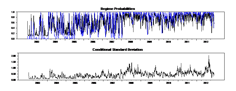
figure 5.png (28.08 KiB) Viewed 45431 times

Here is the code:

Code: Select all

All of this was out of Gray's paper, "Modeling the conditional
* distribution of interest rates as a regime-switching process", J. of
* Financial Economics 42, 1996, pp 27-62.
*
* Revision Schedule:
*   01/2005 Written by Tom Doan, Estima
*   09/2005 Comments added. Changed to use new %MSSMOOTH procedure
*
OPEN DATA data.xlsx
CALENDAR(D) 2003:1:2
all 2012:12:06
DATA(FORMAT=XLSX,ORG=COLUMNS) 2003:01:02 2012:12:06 rupee rate
set rate = rate*100.0
diff rate / drate
spgraph(vfields=2,window="Figure 3")
graph(header="One Month T-Bill Rates")
# rate
graph(header="One Month T-Bill Yields")
# drate
spgraph(done)
*
* This makes extensive use of the Markov switching functions and
* procedures from MSSetup.src
*
@MSSetup(states=2)
*
* The P and Q values in Gray's notation are handled in MSSetup as an M-1
* x M matrix (called P here), with P(i,j) giving the probabilities of
* moving from state j to state i. The Mth row is implicit, as it's just
* the 1-sum of rest of the column.
*
*******************************************************************************
*
* Table 1 information
*
stats drate
cmom(corr,print)
# drate rate{1}
*******************************************************************************
*
* Table 2 estimates
*
* Single regime is linear regression
*
linreg(robust) drate
# constant drate{1}
*
* We're going to use these later for initial conditions
*
compute olsvar =%seesq
compute olsbeta=%beta
*
* Constant variance regime switching model
* This uses Gray's notation for all the variables other than "P"
*
nonlin a01 a02 a11 a12 b01 b02 p
*
* Initial guess values for MS models are always a bit tricky because the
* model isn't globally identified. This is starting with OLS results for
* state 1 and 0 mean coefficients for state 2.
*
compute a01=olsbeta(1),a11=olsbeta(2),b01=sqrt(olsvar)
compute a02=a12=0.0,b02=b01
*
* The p matrix is initialized to make both states fairly persistent.
* (The 2,2 transition is 1-.1=.9).
*
compute p=||.8,.1||
*
* SimpleRegimeF returns the 2-vector of densities in the two regimes. It
* is specific to the data series used (dependent variable <<drate>>) and
* the precise parameterization, and so would need to be altered slightly
* for a different application. Note that this needs to return the actual
* density, not its log.
*
function SimpleRegimeF t
type vector SimpleRegimeF
type integer t
*
compute SimpleRegimeF=||%density((drate(t)-a01-a11*rate(t-1))/b01)/b01,$
                        %density((drate(t)-a02-a12*rate(t-1))/b02)/b02||
end
*
* This is the standard log likelihood FRML for a Markov switching model.
*
frml logl = f=SimpleRegimeF(t),fpt=%MSProb(t,f),log(fpt)
@MSFilterInit
maximize(start=(pstar=%MSInit()),method=bfgs,iters=100,pmethod=simplex,piters=5) logl 2 2012:12:06
*
* It's not clear what residuals are used for the diagonostics for the
* regime switching model. The standardized residuals weighted by the ex
* ante probabilities of the two states seem to give LB's which are
* fairly close to those in the paper.
*
set ustd = %dot(pt_t1,||(drate-a01-a11*drate{1})/b01,(drate-a02-a12*drate{1})/b02||)
graph
# ustd
set usqr = ustd^2
@regcorrs(report,number=15) usqr
*
* Compute the smoothed probabilities and the ex ante probabilities
*
@MSSmoothed %regstart() %regend() psmooth
set exante %regstart() %regend() = pt_t1(t)(1)
set smooth %regstart() %regend() = psmooth(t)(1)
*
* And the conditional standard deviation
*
set condstddev = sqrt(exante*b01^2+(1-exante)*b02^2)
*
spgraph(vfields=2,window="Figure 4")
graph(max=1.0,header="Regime Probabilities") 2
# exante
# smooth
graph(header="Conditional Standard Deviation")
# condstddev
spgraph(done)
*******************************************************************************
*
* Table 3 estimates
*
* Single regime GARCH model
*
garch(p=1,q=1,reg,resids=u,hseries=h) / drate
# constant drate{1}
compute onestate=%beta
*
set usqr = u^2/h
@regcorrs(number=15,report) usqr
*
* Regime-switching GARCH
*
nonlin a01 a02 a11 a12 b01 b11 b21 b02 b12 b22 p
compute a01=%beta(1),a11=%beta(2),b01=olsvar,b11=0.0,b21=0.0
compute a02=%beta(1),a12=%beta(2),b02=%beta(3),b12=%beta(4),b22=%beta(5)
compute p=||.95,.05||
*
set uu = olsvar
set h  = olsvar
*
* RegimeGARCHF returns the 2 vector of densities in the two regimes.
* Again, many lines in this are specific to the problem at hand.
*
function RegimeGARCHF t
type vector RegimeGARCHF
type integer t
local real hh1 hh2 mu1 mu2 mu
*
* Compute state dependent variances
*
compute hh1=b01+b11*uu(t-1)+b21*h(t-1)
compute hh2=b02+b12*uu(t-1)+b22*h(t-1)
*
* Compute state dependent means
*
compute mu1=a01+a11*rate(t-1)
compute mu2=a02+a12*rate(t-1)
*
* Compute the return vector (densities in the two states)
*
compute RegimeGARCHF=||%density((drate(t)-mu1)/sqrt(hh1))/sqrt(hh1),$
                       %density((drate(t)-mu2)/sqrt(hh2))/sqrt(hh2)||
*
* Compute the values of uu (squared residual) and h (variance) to be
* used for the period following.
*
compute mu=mu1*pstar(1)+mu2*pstar(2)
compute uu(t)=(drate(t)-mu)^2
compute h(t)=pstar(1)*(mu1^2+hh1)+pstar(2)*(mu2^2+hh2)-mu^2
end
*
frml logl = f=RegimeGARCHF(t),fpt=%MSProb(t,f),log(fpt)
*
* This combination is able to locate Gray's results - the first MAXIMIZE
* works with the "p" matrix fixed at a fairly high level of persistence,
* and tries to get estimates which separate the two states. The second
* then adds the p matrix to the parmset.
*
nonlin a01 a02 a11 a12 b01 b11 b21 b02 b12 b22
maximize(start=(pstar=%MSInit()),method=bfgs,iters=100,pmethod=simplex,piters=50) logl 2 2012:12:06
nonlin a01 a02 a11 a12 b01 b11 b21 b02 b12 b22 p
maximize(start=(pstar=%MSInit()),method=bfgs,iters=100) logl 2 2012:12:06
*
* Compute the smoothed probabilities and the ex ante probabilities
*
@MSSmoothed %regstart() %regend() psmooth
set exante %regstart() %regend() = pt_t1(t)(1)
set smooth %regstart() %regend() = psmooth(t)(1)
*
* And the conditional standard deviation
*
set condstddev = sqrt(h)
*
spgraph(vfields=2,window="Figure 5")
graph(max=1.0,header="Regime Probabilities") 2
# exante
# smooth
graph(header="Conditional Standard Deviation")
# condstddev
spgraph(done)
*
*
* However, this set of initial guess values (which are actually the
* result of a typo in trying to reproduce the article's numbers) find a
* local max with quite a bit higher likelihood, and dramatically
* different behavior. How one might find this systematically is unclear.
*
compute a01=.1407,a02=-.0011,a11=-.0141,a12=.0006,b01=.0004,b11=.4609,b21=.1977,b02=.0099,b12=.1655,b22=.2685,p=||.9739,1-.9896||
maximize(start=(pstar=%MSInit()),method=bfgs,iters=100,pmethod=simplex,piters=50) logl 2 2012:12:06
*******************************************************************************

[TomDoan]

You realize the Gray was analyzing US interest rates and his model was chosen for that. I have no idea what your series is, but it has very different dynamics than Gray's. Your results suggest that your mean model is wrong---you're showing signs of overdifferencing.

There's absolutely nothing wrong with a small P(1,2), that means P(2,2) is fairly large, so both regimes are persistent, which isn't that unusual. However, it looks like a MS model is overkill. There appears to be a structural break about at the midpoint of your sample, and the MS is simply picking that up.

[jack]

Dear Tom,
I adjusted the model and here is the result. My data is exchange rate return. In the first regime, there is negative first order correlation (A11) but it is positive in the second regime (A12). And in the simple model here isn't any correlation. Isn't it strange?

Statistics on Series RATE
Daily(5) Data From 2003:01:02 To 2012:12:06
Observations                  2591
Sample Mean               0.009871      Variance                   0.254899
Standard Error            0.504875      SE of Sample Mean          0.009919
t-Statistic (Mean=0)      0.995250      Signif Level (Mean=0)      0.319708
Skewness                  0.204085      Signif Level (Sk=0)        0.000022
Kurtosis (excess)         5.843007      Signif Level (Ku=0)        0.000000
Jarque-Bera            3703.762694      Signif Level (JB=0)        0.000000


Correlation Matrix
            RATE       RATE{1}
RATE    1.0000000000 0.0119264167
RATE{1} 0.0119264167 1.0000000000


Linear Regression - Estimation by Least Squares
With Heteroscedasticity-Consistent (Eicker-White) Standard Errors
Dependent Variable RATE
Daily(5) Data From 2003:01:03 To 2012:12:06
Usable Observations                      2590
Degrees of Freedom                       2588
Centered R^2                        0.0001422
R-Bar^2                            -0.0002441
Uncentered R^2                      0.0005240
Mean of Dependent Variable       0.0098672569
Std Error of Dependent Variable  0.5049725654
Standard Error of Estimate       0.5050341946
Sum of Squared Residuals         660.09408372
Log Likelihood                     -1904.7459
Durbin-Watson Statistic                1.9986

    Variable                        Coeff      Std Error      T-Stat      Signif
************************************************************************************
1.  Constant                     0.0097490582 0.0098791820      0.98683  0.32372673
2.  RATE{1}                      0.0119265083 0.0328551991      0.36300  0.71660327


MAXIMIZE - Estimation by BFGS
Convergence in     9 Iterations. Final criterion was  0.0000046 <=  0.0000100
Daily(5) Data From 2003:01:03 To 2012:12:06
Usable Observations                      2590
Function Value                     -1233.4961

    Variable                        Coeff      Std Error      T-Stat      Signif
************************************************************************************
1.  A01                           0.034375380  0.018717432      1.83654  0.06627729
2.  A02                          -0.018159015  0.005528836     -3.28442  0.00102193
3.  A11                           0.012948320  0.025544213      0.50690  0.61222612
4.  A12                          -0.036714468  0.030673547     -1.19694  0.23132901
5.  B01                           0.676243274  0.014175432     47.70530  0.00000000
6.  B02                           0.178091226  0.005170468     34.44393  0.00000000
7.  P(1,1)                        0.964435901  0.006035214    159.80145  0.00000000
8.  P(1,2)                        0.038300888  0.005961810      6.42437  0.00000000

Lag  Corr  Partial   LB Q    Q Signif
  1 0.0339  0.0339  2.988551    0.0839
  2 0.0330  0.0319  5.815595    0.0546
  3 0.0209  0.0188  6.950812    0.0735
  4 0.0580  0.0558 15.691318    0.0035
  5 0.0679  0.0634 27.684503    0.0000
  6 0.0430  0.0356 32.499693    0.0000
  7 0.0521  0.0445 39.564417    0.0000
  8 0.0292  0.0194 41.786765    0.0000
  9 0.0177  0.0056 42.605573    0.0000
 10 0.0320  0.0206 45.269952    0.0000
 11 0.0659  0.0541 56.593080    0.0000
 12 0.0233  0.0090 58.003813    0.0000
 13 0.0301  0.0184 60.358844    0.0000
 14 0.0519  0.0414 67.379388    0.0000
 15 0.0336  0.0184 70.331039    0.0000


GARCH Model - Estimation by BFGS
Convergence in    23 Iterations. Final criterion was  0.0000041 <=  0.0000100
Dependent Variable RATE
Daily(5) Data From 2003:01:03 To 2012:12:06
Usable Observations                      2590
Log Likelihood                     -1106.0489

    Variable                        Coeff      Std Error      T-Stat      Signif
************************************************************************************
1.  Constant                     -0.009116152  0.004583112     -1.98907  0.04669295
2.  RATE{1}                       0.035172878  0.022646726      1.55311  0.12039663

3.  C                             0.001088115  0.000282215      3.85562  0.00011543
4.  A                             0.246598747  0.026254036      9.39279  0.00000000
5.  B                             0.791129966  0.018299852     43.23150  0.00000000

Lag  Corr  Partial   LB Q    Q Signif
  1  0.053   0.053  7.155283    0.0075
  2 -0.008  -0.011  7.314639    0.0258
  3 -0.024  -0.023  8.800338    0.0321
  4  0.032   0.035 11.463173    0.0218
  5 -0.005  -0.009 11.533096    0.0418
  6 -0.030  -0.030 13.918315    0.0306
  7 -0.030  -0.025 16.257684    0.0229
  8 -0.024  -0.023 17.751739    0.0232
  9 -0.031  -0.030 20.225390    0.0166
 10 -0.016  -0.012 20.850930    0.0222
 11 -0.026  -0.025 22.658262    0.0197
 12 -0.019  -0.018 23.600898    0.0230
 13 -0.027  -0.026 25.444931    0.0202
 14 -0.039  -0.040 29.388071    0.0093
 15 -0.037  -0.036 32.917932    0.0048


MAXIMIZE - Estimation by BFGS
Convergence in     2 Iterations. Final criterion was  0.0000050 <=  0.0000100
Daily(5) Data From 2003:01:03 To 2012:12:06
Usable Observations                      2590
Function Value                     -1054.0329

    Variable                        Coeff      Std Error      T-Stat      Signif
************************************************************************************
1.  A01                           0.013549085  0.012540572      1.08042  0.27995519
2.  A02                          -0.014930348  0.004370346     -3.41629  0.00063482
3.  A11                           0.064567104  0.029604611      2.18098  0.02918480
4.  A12                          -0.064066500  0.034049382     -1.88158  0.05989361
5.  B01                           0.067479479  0.005412803     12.46664  0.00000000
6.  B11                           0.135819468  0.013344841     10.17768  0.00000000
7.  B21                           0.808728790  0.017795344     45.44609  0.00000000
8.  B02                           0.003753066  0.000429312      8.74204  0.00000000
9.  B12                           0.312228200  0.047843182      6.52608  0.00000000
10. B22                           0.294668993  0.019177199     15.36559  0.00000000


MAXIMIZE - Estimation by BFGS
Convergence in    22 Iterations. Final criterion was  0.0000006 <=  0.0000100
Daily(5) Data From 2003:01:03 To 2012:12:06
Usable Observations                      2590
Function Value                     -1049.7041

    Variable                        Coeff      Std Error      T-Stat      Signif
************************************************************************************
1.  A01                           0.010332656  0.012722085      0.81218  0.41668686
2.  A02                          -0.015752333  0.004410645     -3.57144  0.00035503
3.  A11                           0.066010875  0.030439228      2.16861  0.03011215
4.  A12                          -0.086271210  0.037563514     -2.29668  0.02163728
5.  B01                           0.050481058  0.009854571      5.12260  0.00000030
6.  B11                           0.156253488  0.032079328      4.87085  0.00000111
7.  B21                           0.805724006  0.051333920     15.69574  0.00000000
8.  B02                           0.003278824  0.001207730      2.71487  0.00663027
9.  B12                           0.229633335  0.069779573      3.29084  0.00099889
10. B22                           0.249913547  0.039345596      6.35175  0.00000000
11. P(1,1)                        0.959801475  0.014292487     67.15427  0.00000000
12. P(1,2)                        0.076891035  0.021664827      3.54912  0.00038652


MAXIMIZE - Estimation by BFGS
NO CONVERGENCE IN 24 ITERATIONS
LAST CRITERION WAS  0.0000000
SUBITERATIONS LIMIT EXCEEDED.
ESTIMATION POSSIBLY HAS STALLED OR MACHINE ROUNDOFF IS MAKING FURTHER PROGRESS DIFFICULT
TRY HIGHER SUBITERATIONS LIMIT, TIGHTER CVCRIT, DIFFERENT SETTING FOR EXACTLINE OR ALPHA ON NLPAR
RESTARTING ESTIMATION FROM LAST ESTIMATES OR DIFFERENT INITIAL GUESSES MIGHT ALSO WORK
Daily(5) Data From 2003:01:03 To 2012:12:06
Usable Observations                      2590
Function Value                     -1009.2015

    Variable                        Coeff      Std Error      T-Stat      Signif
************************************************************************************
1.  A01                          -0.019277002  0.000748007    -25.77117  0.00000000
2.  A02                           0.029994572  0.000048554    617.75949  0.00000000
3.  A11                          -0.134259201  0.001260581   -106.50579  0.00000000
4.  A12                           0.526709694  0.050463318     10.43748  0.00000000
5.  B01                          -0.001186886  0.000009806   -121.03180  0.00000000
6.  B11                           0.081255446  0.002636271     30.82211  0.00000000
7.  B21                           0.523741479  0.003905943    134.08835  0.00000000
8.  B02                           0.016741849  0.000448428     37.33451  0.00000000
9.  B12                           0.070595091  0.019397509      3.63939  0.00027329
10. B22                           1.679419320  0.037539345     44.73758  0.00000000
11. P(1,1)                        0.746300187  0.000065127  11459.07867  0.00000000
12. P(1,2)                        0.611475906  0.015966929     38.29640  0.00000000

Following figure shows ex ante and smoothed probabilities. Introduction of exchange rate futures took place on April 23, 1990 . Can one say that this event has increased the volatility of market? Or it has had a destabilizing effect on the market?
Can I have this figure to be shaded after this time? How can I have LB statistic for squared residuals of Regime-switching GARCH?

figure 5.png (27.54 KiB) Viewed 45421 times

[TomDoan]

If something happened in April 1990 and your data set starts in 2003, how do you think that your results will show anything?

[Catife]

Dear Tom,

I have some questions about the part of time-varying transition probabilities (TVTP) in the sample codes.

The first question is about the calculations of pt_t, pt_t1, and smoothed probabilities after estimating the TVTP model of Gray (1996). Based on my understanding, hamilton filter still works in this case since Gray (1996)'s TVTP setup is still based on lagged information. However, when I estimate the TVTP part, I find the calculated pt_t, pt-t1, and smoothed probabilities are not informative in terms of that they fluctuate around 0.3-0.4 for one regime over time. Are these proper outcomes or the hamilton filter should be changed accordingly in this case?

The second question is the difference between Filardo (1994) and Gray (1996) regarding the TVTP parts of them. In the sample codes of Filardo (1994) you provided, there is a formal function (%msvarpmat) which is re-defined to accommodate TVTP in the codes. On the other hand, the sample codes of Gary (1996) only override the transition matrix when we formulate the likelihood function. Is there a reason to set up TVTP differently, given the TVTP are defined similarly in these two papers from my view?

I will appreciate your replies and comments. Thank you very much.

Best Regards

[jack]

I'm really sorry. The event took place in April, 2008.

[TomDoan]

If you have a particular date of interest, why are you doing a MS model? That's completely wrong for that. Just concentrate on the differences in the model before and after the policy change.