Balcilar Gupta Miller EE 2015

This is based upon Balcilar, Gupta, Miller(2015). It estimates a Markov Switching VECM on log stock prices (LSP) and log oil price (LOIL). This assumes a cointegrating vector fixed between regimes, but different VECM coefficients and covariance matrices.

This does a couple of things differently from the original paper. First, it scales up the values of the log by 100 to give better scale to the variances. (As with GARCH models, when the variances are being estimated as parameters, it helps to get their scales up several orders of magnitude):

set loil = 100.0*loil

set lsp = 100.0*lsp

More important, it "fuzzes" up the zero values of dloil. There are so many of these (often in a row) that the MS model can achieve an infinite log likelihood by zeroing out the coefficients on everything other than the lagged dloil in one regime to achieve a perfect fit there. This doesn't really change the results in any meaningful way, but avoids numerical problems. (This was not done in the paper and wouldn't need to be done in other data that didn't have the large number of true zeros for one of the series). This is only necessary for the EM or ML estimation—the Bayesian estimation has a prior which prevents the variances from going all the way to zero.

Note that this is a very technically demanding type of model even without the behavior of the log oil price. The types of issues that come up with these are covered in detail as part of the Structural Breaks and Switching Models course.

set dloil = %if(dloil==0.0,%ran(.1),dloil)

The cointegrating vector is estimated using @JOHMLE. The cointegrating vector is normalized to a unit coefficient on LOIL.

compute varlags=2

@johmle(lags=varlags,det=constant,cv=cv)

# lsp loil

* Normalize to a unit coefficient on oil

compute cv=cv/cv(2)

* This is the error correction series

set ect = cv(1)*lsp+cv(2)*loil

equation(coeffs=cv) ecteq *

# lsp loil

The output from @JOHMLE is shown here. This very strongly suggests one unit root between the two series; since both are fairly clearly non-stationary, this means they are cointegrated.

The MSVECM is then set up with @MSSysRegression with the differences as the dependent variables, with lagged differences, CONSTANT and the lagged error correction term as the regressors. VARLAGS was set above to the number of lags on the unrestricted VAR, so this requires 1 less on the lagged differences. Both coefficients and the covariance matrix are allowed to switch between regimes (SWITCH=CH option). Note that the order of the variables in the @MSSysRegression should match the order that variables are included in the fixed coefficient VECM that follows (lagged differences in order, followed by deterministics and finally the error correction term).

@mssysregression(regimes=2,switch=ch)

# dlsp dloil

# dlsp{1 to varlags-1} dloil{1 to varlags-1} constant ect{1}

This sets up an estimates the fixed coefficient VECM.

system(model=vecm)

variables lsp loil

lags 1 to varlags

det constant

ect ecteq

end(system)

estimate

The output from the ESTIMATE is here. The EC1{1} coefficients show the adjustment coefficients: the main interpretation is that (in a fixed VECM) the oil price does most of the adjustment back towards equilibrium.

In the MSVECM, the expected "labeling" of regimes is that regime 1 will be the low volatility and regime 2 the high volatility. This pushes the guess values in that direction, and then runs the EM algorithm for 100 iterations (only about 50 turn out to be needed to get convergence).

* Use the sample range from the full system

compute gstart=%regstart(),gend=%regend()

@MSSysRegInitial gstart gend

* Try to enforce regime 1 as having lower volatility

compute sigmav(1)=.25*sigmav(1)

compute sigmav(2)=4.0*sigmav(2)

@MSSysRegEMGeneralSetup

do emits=1,100

@MSSysRegEMStep gstart gend

disp "Iteration" emits "Log likelihood" %logl

end do emits

This does 10 iterations of BHHH to allow calculation of standard errors for the estimates. This first sets up the parameter sets and initializes the regime probability matrices (required for ML, but not EM, which uses its own).

@MSSysRegParmset(parmset=regparms)

nonlin(parmset=msparms) p

compute p=%xsubmat(p,1,nregimes-1,1,nregimes)

frml logl = f=%MSSysRegFVec(t),fpt=%MSProb(t,f),log(fpt)

@MSFilterInit

maximize(start=$

%(logdet=%MSSysRegInitVariances(),pstar=%MSSysRegInit()),$

parmset=regparms+msparms,method=bhhh,iters=10) logl gstart gend

Note that this (see output) comes up with quite a bit smaller a log likelihood than is shown in the paper. This is because of the "fuzzing" of the data. (For the same reason, the log likelihood will be slightly different from run to run. If you want exactly reproducible results, you need to use the SEED instruction at the top of the program to control the random numbers). Without the fuzzing, the log likelihood actually has a spike to infinity (which is bad), and is only finite because of some limits on the numerical calculations. Again, this is only necessary because of the nature of the oil data.

Note also that the BHHH estimates don't "converge". This is intentional—BHHH is being used solely to get estimated standard errors on the coefficients.

This computes and graphs the smoothed probabilities of the low and high volatility regimes.

@MSSmoothed gstart gend psmooth

* Smoothed probabilities of the regimes

set p1smooth = psmooth(t)(1)

graph(footer="Smoothed Probabilities of Low Volatility Regime",max=1.0,min=0.0)

# p1smooth

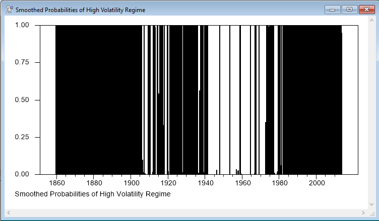
set p2smooth = 1-p1smooth

graph(footer="Smoothed Probabilities of High Volatility Regime",max=1.0,min=0.0)

# p2smooth

The two graphs add up to one, and might reasonably be presented together as a stacked bar graph, but given the number of data points and the number of very short-term but almost complete regime switches, that would end up being hard to read—note, for instance, that the high-volatility regime seems to be solid from roughly 1860-1905, but when you look at the low-volatility regime, there are a few time periods which are in that regime, but at this screen resolution, they aren't visible against the black.

The Bayesian estimation (to generate regime-dependent impulse responses with error bands) is very similar to that from Ehrmann, Ellison and Valla. The steps followed are

1.Draw the (regime-specific) covariance matrices given the VECM coefficients and regimes. This involves a (mild) shrinkage towards a common covariance matrix.

2.Draw the VECM coefficients given the covariance matrices and regimes.

3.Because it's possible (though unlikely in this case) that the draw for the regime-specific covariance might cause the order to reverse from the one desired (where regime 1 has lower oil variance), the various statistics are ordered to match the intended labeling.

4.Draw the regimes. If one regime has too few time periods, redraw.

5.Draw the transition probabilities.

One big difference from EEV is that the data set is much larger, so the minimum regime size is set quite a bit higher (here 100).

A second difference with EEV is to deal with the fact that this is a VECM while the EEV paper is just a VAR. There's no difference in drawing coefficients due to it being a VECM, but there is a difference in computing impulse responses as the error correction term is endogenous, so the IMPULSE instructions use MODEL=VECM (the VECM model defined above) and the regime-specific coefficients are placed into the VECM model. Note that this is using not the typical Cholesky factor of the covariance matrices, but a standardized Cholesky factor which has unit own impacts for both the components. (Eliminate the factor=%ddivide(...) calculations in each of these to use the more common Cholesky factor). The resulting IRF's will not show the (rather considerable) difference in variances between regimes, but only the difference in the shape of the responses.

@MSSysRegSetModel(regime=1)

compute factor=%decomp(sigmav(1)),factor=%ddivide(factor,%xdiag(factor))

compute %modelsetcoeffs(vecm,%modelgetcoeffs(MSSysRegModel))

impulse(noprint,model=vecm,results=impulses1,steps=steps,factor=factor)

* Save IRF's for regime 2

@MSSysRegSetModel(regime=2)

compute factor=%decomp(sigmav(2)),factor=%ddivide(factor,%xdiag(factor))

compute %modelsetcoeffs(vecm,%modelgetcoeffs(MSSysRegModel))

impulse(noprint,model=vecm,results=impulses2,steps=steps,factor=factor)

The following is used to "interleave" the two sets of responses, giving what are in effect four shocks: in order, the stock and oil shocks in regime 1 and the stock and oil shocks in regime 2.

dim %%responses(draw)(%rows(impulses1)*%cols(impulses1)*2,steps)

ewise %%responses(draw)(i,j)=ix=%vec(%xt(impulses1,j)~~%xt(impulses2,j)),ix(i)

Outside the MCMC loop, the sampled parameters are processed using @MCMCPOSTPROC:

@mcmcpostproc(ndraws=ndraws,mean=bmeans,stderrs=bstderrs) bgibbs

report(action=define)

report(atrow=1,atcol=1,fillby=cols) %parmslabels(allparms)

report(atrow=1,atcol=2,fillby=cols) bmeans

report(atrow=1,atcol=3,fillby=cols) bstderrs

report(action=format,picture="*.########")

report(action=show)

The output of this (with the means and standard errors from the simulations) are shown in a table.

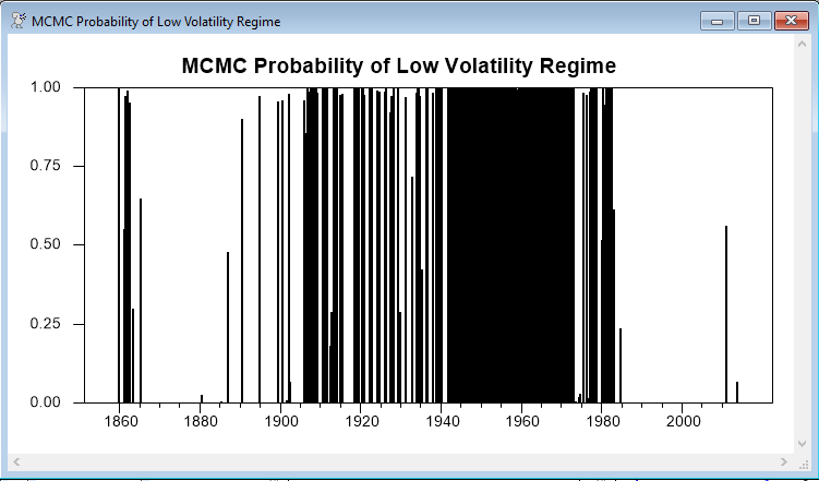
The following converts the counts of the regimes across simulations into the regime probabilities. This should be (and by inspection are) very similar to the smoothed probabilities at the point estimates.

set regime1 gstart gend = regime1/ndraws

graph(header="MCMC Probability of Low Volatility Regime",$

style=bar,min=0.0,max=1.0)

# regime1

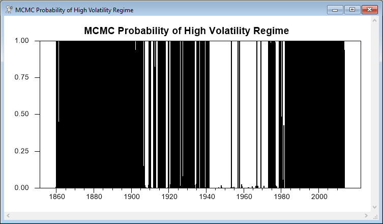
set regime2 = 1-regime1

graph(header="MCMC Probability of High Volatility Regime",$

style=bar,min=0.0,max=1.0)

# regime2

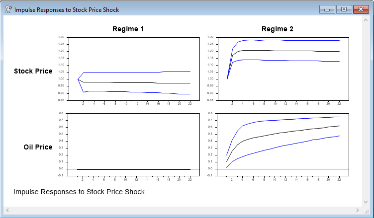
Finally, this uses @MCProcessIRF to process the draws, in this case with the .05 and .95 percentiles for the lower and upper bounds. The labels here would need to be changed for a different application. The graphs are shown here. Note that, by construction (because of the use of scaled Cholesky factors), the impacts to own shocks are 1.0 in each regime and the impact of the oil price shock on stocks is zero (as oil prices were second in the Cholesky ordering). Regime 1 basically picks out the periods where the oil price wasn't changing, so the responses are flat.

@MCProcessIRF(model=vecm,lower=lower,upper=upper,irf=irf,percentiles=||.05,.95||)

***************************

*** CHANGE FOLLOWING LABELS

***************************

compute ylab = ||"Stock Price","Oil Price"||

compute xlab = ||"Regime 1","Regime 2","Regime 1","Regime 2"||

compute shocklab = ||"Stock Price Shock","Stock Price Shock","Oil Price Shock","Oil Price Shock"||

compute nshock = 2*nvar

do var=1,nvar

do shock=1,nshock

display "Response of" ylab(1,var) "to" shocklab(1,shock) "in" xlab(1,shock)

print(number=0) / irf(var,shock) lower(var,shock) upper(var,shock)

end do

* CHANGE labels here

spgraph(footer="Impulse Responses to Stock Price Shock",vfields=nvar,hfields=2,$

xlabels=||"Regime 1","Regime 2"||,ylabels=ylab)

do var=1,nvar

table(noprint) / lower(var,1) upper(var,1) lower(var,2) upper(var,2)

do shock=1,2

graph(row=var,col=shock,max=%maximum,min=%minimum,nodates) 3

# irf(var,shock)

# lower(var,shock) / 2

# upper(var,shock) / 2

end do shock

end do var

spgraph(done)

spgraph(footer="Impulse Responses to Oil Price Shock",vfields=nvar,hfields=2,$

xlabels=||"Regime 1","Regime 2"||,ylabels=ylab)

do var=1,nvar

table(noprint) / lower(var,3) upper(var,3) lower(var,4) upper(var,4)

do shock=3,4

graph(row=var,col=shock-2,max=%maximum,min=%minimum,nodates) 3

# irf(var,shock)

# lower(var,shock) / 2

# upper(var,shock) / 2

end do shock

end do var

spgraph(done)

Output

Likelihood Based Analysis of Cointegration

Variables: LSP LOIL

Estimated from 1859:11 to 2013:12

Data Points 1850 Lags 2 with Constant

Unrestricted eigenvalues, -T log(1-lambda) and Trace Test

Roots Rank EigVal Lambda-max Trace Trace-95%

2 0 0.0174 32.5131 32.7758 15.3400

1 1 0.0001 0.2627 0.2627 3.8400

Cointegrating Vector for Largest Eigenvalue

LSP LOIL

-0.009457 0.014157

VAR/System - Estimation by Cointegrated Least Squares

Monthly Data From 1859:11 To 2013:12

Usable Observations 1850

Dependent Variable LSP

Mean of Dependent Variable 0.3851703594

Std Error of Dependent Variable 4.7724295649

Standard Error of Estimate 4.7424864118

Sum of Squared Residuals 41518.713417

Durbin-Watson Statistic 1.9952

Variable Coeff Std Error T-Stat Signif

************************************************************************************

1. D_LSP{1} 0.1178455473 0.0231553141 5.08935 0.00000040

2. D_LOIL{1} 0.0023297588 0.0122372542 0.19038 0.84903036

3. Constant 0.4261814886 0.1696970408 2.51143 0.01210925

4. EC1{1} 0.0010459224 0.0015609335 0.67006 0.50290200

Dependent Variable LOIL

Mean of Dependent Variable 0.0856114791

Std Error of Dependent Variable 9.0282969307

Standard Error of Estimate 8.2620875079

Sum of Squared Residuals 126011.81812

Durbin-Watson Statistic 1.9950

Variable Coeff Std Error T-Stat Signif

************************************************************************************

1. D_LSP{1} 0.062857910 0.040339859 1.55821 0.11935525

2. D_LOIL{1} 0.383850229 0.021319042 18.00504 0.00000000

3. Constant -1.236265136 0.295636440 -4.18171 0.00003029

4. EC1{1} -0.015324416 0.002719369 -5.63528 0.00000002

Iteration 1 Log likelihood -11560.64083

Iteration 2 Log likelihood -11307.83080

Iteration 3 Log likelihood -11254.97136

Iteration 4 Log likelihood -11233.57797

Iteration 5 Log likelihood -11219.97211

Iteration 6 Log likelihood -11207.71036

Iteration 7 Log likelihood -11195.07878

Iteration 8 Log likelihood -11181.62356

Iteration 9 Log likelihood -11166.88144

Iteration 10 Log likelihood -11148.62961

Iteration 11 Log likelihood -11120.87984

Iteration 12 Log likelihood -11069.60003

Iteration 13 Log likelihood -10981.82451

Iteration 14 Log likelihood -10883.82862

Iteration 15 Log likelihood -10768.48378

Iteration 16 Log likelihood -10637.96780

Iteration 17 Log likelihood -10483.31751

Iteration 18 Log likelihood -10363.24138

Iteration 19 Log likelihood -10261.28957

Iteration 20 Log likelihood -10203.16957

Iteration 21 Log likelihood -10183.82368

Iteration 22 Log likelihood -10178.96246

Iteration 23 Log likelihood -10177.20786

Iteration 24 Log likelihood -10173.55862

Iteration 25 Log likelihood -10160.36846

Iteration 26 Log likelihood -10147.99089

Iteration 27 Log likelihood -10139.00867

Iteration 28 Log likelihood -10122.41796

Iteration 29 Log likelihood -10055.32525

Iteration 30 Log likelihood -10025.39302

Iteration 31 Log likelihood -10006.93886

Iteration 32 Log likelihood -9997.43512

Iteration 33 Log likelihood -9997.12738

Iteration 34 Log likelihood -9997.11744

Iteration 35 Log likelihood -9997.11699

Iteration 36 Log likelihood -9997.11695

Iteration 37 Log likelihood -9997.11694

Iteration 38 Log likelihood -9997.11693

Iteration 39 Log likelihood -9997.11693

Iteration 40 Log likelihood -9997.11693

Iteration 41 Log likelihood -9997.11693

Iteration 42 Log likelihood -9997.11693

Iteration 43 Log likelihood -9997.11693

Iteration 44 Log likelihood -9997.11693

Iteration 45 Log likelihood -9997.11693

Iteration 46 Log likelihood -9997.11693

Iteration 47 Log likelihood -9997.11693

Iteration 48 Log likelihood -9997.11693

Iteration 49 Log likelihood -9997.11693

Iteration 50 Log likelihood -9997.11693

Iteration 51 Log likelihood -9997.11693

Iteration 52 Log likelihood -9997.11693

Iteration 53 Log likelihood -9997.11693

Iteration 54 Log likelihood -9997.11693

Iteration 55 Log likelihood -9997.11693

Iteration 56 Log likelihood -9997.11693

Iteration 57 Log likelihood -9997.11693

Iteration 58 Log likelihood -9997.11693

Iteration 59 Log likelihood -9997.11693

Iteration 60 Log likelihood -9997.11693

Iteration 61 Log likelihood -9997.11693

Iteration 62 Log likelihood -9997.11693

Iteration 63 Log likelihood -9997.11693

Iteration 64 Log likelihood -9997.11693

Iteration 65 Log likelihood -9997.11693

Iteration 66 Log likelihood -9997.11693

Iteration 67 Log likelihood -9997.11693

Iteration 68 Log likelihood -9997.11693

Iteration 69 Log likelihood -9997.11693

Iteration 70 Log likelihood -9997.11693

Iteration 71 Log likelihood -9997.11693

Iteration 72 Log likelihood -9997.11693

Iteration 73 Log likelihood -9997.11693

Iteration 74 Log likelihood -9997.11693

Iteration 75 Log likelihood -9997.11693

Iteration 76 Log likelihood -9997.11693

Iteration 77 Log likelihood -9997.11693

Iteration 78 Log likelihood -9997.11693

Iteration 79 Log likelihood -9997.11693

Iteration 80 Log likelihood -9997.11693

Iteration 81 Log likelihood -9997.11693

Iteration 82 Log likelihood -9997.11693

Iteration 83 Log likelihood -9997.11693

Iteration 84 Log likelihood -9997.11693

Iteration 85 Log likelihood -9997.11693

Iteration 86 Log likelihood -9997.11693

Iteration 87 Log likelihood -9997.11693

Iteration 88 Log likelihood -9997.11693

Iteration 89 Log likelihood -9997.11693

Iteration 90 Log likelihood -9997.11693

Iteration 91 Log likelihood -9997.11693

Iteration 92 Log likelihood -9997.11693

Iteration 93 Log likelihood -9997.11693

Iteration 94 Log likelihood -9997.11693

Iteration 95 Log likelihood -9997.11693

Iteration 96 Log likelihood -9997.11693

Iteration 97 Log likelihood -9997.11693

Iteration 98 Log likelihood -9997.11693

Iteration 99 Log likelihood -9997.11693

Iteration 100 Log likelihood -9997.11693

MAXIMIZE - Estimation by BHHH

NO CONVERGENCE IN 10 ITERATIONS

LAST CRITERION WAS 0.0000282

TRY INCREASING ITERS OPTION

Monthly Data From 1859:11 To 2013:12

Usable Observations 1850

Function Value -9997.1146

Variable Coeff Std Error T-Stat Signif

************************************************************************************

1. BETASYS(1)(1,1) -0.0247374 0.0332716 -0.74350 0.45717918

2. BETASYS(1)(2,1) -0.1009958 0.0451721 -2.23580 0.02536480

3. BETASYS(1)(3,1) 0.6079702 0.2657660 2.28761 0.02215997

4. BETASYS(1)(4,1) 0.0005496 0.0023670 0.23219 0.81638886

5. BETASYS(1)(1,2) 0.0006372 0.0009700 0.65694 0.51121807

6. BETASYS(1)(2,2) -0.0009533 0.0012910 -0.73838 0.46028351

7. BETASYS(1)(3,2) -0.0081536 0.0075651 -1.07780 0.28112305

8. BETASYS(1)(4,2) -0.0000862 0.0000597 -1.44277 0.14908448

9. BETASYS(2)(1,1) 0.1736360 0.0159838 10.86328 0.00000000

10. BETASYS(2)(2,1) 0.0077599 0.0124969 0.62095 0.53463469

11. BETASYS(2)(3,1) 0.3625191 0.2406150 1.50664 0.13190416

12. BETASYS(2)(4,1) 0.0018177 0.0025009 0.72681 0.46734101

13. BETASYS(2)(1,2) 0.0922228 0.0634165 1.45424 0.14587987

14. BETASYS(2)(2,2) 0.4058672 0.0188731 21.50502 0.00000000

15. BETASYS(2)(3,2) -1.6100505 0.3409264 -4.72258 0.00000233

16. BETASYS(2)(4,2) -0.0227902 0.0032363 -7.04200 0.00000000

17. SIGMAV(1)(1,1) 15.5523822 0.8073017 19.26465 0.00000000

18. SIGMAV(1)(2,1) 0.0130786 0.0177497 0.73684 0.46122123

19. SIGMAV(1)(2,2) 0.0104593 0.0006206 16.85375 0.00000000

20. SIGMAV(2)(1,1) 25.6440133 0.4606679 55.66703 0.00000000

21. SIGMAV(2)(2,1) 2.9535467 1.7255112 1.71169 0.08695312

22. SIGMAV(2)(2,2) 101.6351720 2.0645565 49.22857 0.00000000

23. P(1,1) 0.8520094 0.0150619 56.56708 0.00000000

24. P(1,2) 0.0774763 0.0077890 9.94689 0.00000000

BETASYS(1)(1,1) -0.02463032 0.03981362

BETASYS(1)(2,1) -0.10234106 0.04539403

BETASYS(1)(3,1) 0.61815159 0.30850087

BETASYS(1)(4,1) 0.00059882 0.00250627

BETASYS(1)(1,2) 0.00065533 0.00102024

BETASYS(1)(2,2) -0.00091640 0.00125031

BETASYS(1)(3,2) -0.00841636 0.00805771

BETASYS(1)(4,2) -0.00008871 0.00006467

BETASYS(2)(1,1) 0.17391208 0.02861090

BETASYS(2)(2,1) 0.00762267 0.01351723

BETASYS(2)(3,1) 0.35768116 0.20768441

BETASYS(2)(4,1) 0.00176943 0.00203585

BETASYS(2)(1,2) 0.09116138 0.05766553

BETASYS(2)(2,2) 0.40506192 0.02634086

BETASYS(2)(3,2) -1.60713145 0.40670660

BETASYS(2)(4,2) -0.02277531 0.00417144

SIGMAV(1)(1,1) 15.96444531 0.93738170

SIGMAV(1)(2,1) 0.01326611 0.01760777

SIGMAV(1)(2,2) 0.01128198 0.00069869

SIGMAV(2)(1,1) 25.57182257 1.05392093

SIGMAV(2)(2,1) 2.88621353 1.41274887

SIGMAV(2)(2,2) 99.21558694 3.89277779

P(1,1) 0.85550629 0.01465614

P(2,1) 0.14449371 0.01465614

P(1,2) 0.07619118 0.00835418

P(2,2) 0.92380882 0.00835418

MAXIMIZE - Estimation by BHHH

NO CONVERGENCE IN 10 ITERATIONS

LAST CRITERION WAS 0.0000400

TRY INCREASING ITERS OPTION

Monthly Data From 1859:11 To 2013:12

Usable Observations 1850

Function Value -10010.6080

Variable Coeff Std Error T-Stat Signif

************************************************************************************

1. BETASYS(1)(1,1) -0.0205654 0.0335812 -0.61241 0.54026753

2. BETASYS(1)(2,1) -0.1048061 0.0466288 -2.24767 0.02459726

3. BETASYS(1)(3,1) 0.6021972 0.2684988 2.24283 0.02490778

4. BETASYS(1)(4,1) 0.0005968 0.0023814 0.25062 0.80211104

5. BETASYS(1)(1,2) -0.0000397 0.0010084 -0.03933 0.96862774

6. BETASYS(1)(2,2) -0.0008816 0.0012656 -0.69658 0.48606579

7. BETASYS(1)(3,2) 0.0020406 0.0080302 0.25412 0.79940333

8. BETASYS(1)(4,2) 0.0000213 0.0000660 0.32299 0.74669952

9. BETASYS(2)(1,1) 0.1714348 0.0159532 10.74613 0.00000000

10. BETASYS(2)(2,1) 0.0078668 0.0124651 0.63111 0.52796794

11. BETASYS(2)(3,1) 0.3701234 0.2395740 1.54492 0.12236484

12. BETASYS(2)(4,1) 0.0018398 0.0024917 0.73839 0.46027537

13. BETASYS(2)(1,2) 0.0914785 0.0632947 1.44528 0.14837917

14. BETASYS(2)(2,2) 0.4048954 0.0188295 21.50324 0.00000000

15. BETASYS(2)(3,2) -1.6002946 0.3401767 -4.70430 0.00000255

16. BETASYS(2)(4,2) -0.0226579 0.0032288 -7.01738 0.00000000

17. SIGMAV(1)(1,1) 15.6366840 0.8222880 19.01607 0.00000000

18. SIGMAV(1)(2,1) 0.0108082 0.0181188 0.59652 0.55083073

19. SIGMAV(1)(2,2) 0.0108673 0.0005941 18.29286 0.00000000

20. SIGMAV(2)(1,1) 25.5946801 0.4589739 55.76501 0.00000000

21. SIGMAV(2)(2,1) 2.9558027 1.7193389 1.71915 0.08558693

22. SIGMAV(2)(2,2) 101.4636174 2.0573178 49.31840 0.00000000

23. P(1,1) 0.8549694 0.0150089 56.96399 0.00000000

24. P(1,2) 0.0754364 0.0076743 9.82977 0.00000000

Graphs