|
Statistics and Algorithms / Forecasting (Univariate) / Box-Jenkins (ARIMA) Modeling |
The Box-Jenkins methodology provides a broad range of models for fitting the serial correlation patterns of both seasonal and non-seasonal data. The class of models is rich enough that there is often a choice which fits the data adequately with very few parameters.
The fitting process as described in textbooks (Box, Jenkins, Reinsel (2008), Brockwell and Davis (2002), DeLurgio (1998), Enders (2014), and Granger and Newbold (1986) are among the many worthy examples) is an interactive process between the forecaster and the data. We describe the process here briefly, but you will need to consult an appropriate text if you are new to ARIMA modeling.
Advantages
Box-Jenkins models cover a much larger range of series than exponential smoothing models. They require less data than spectral methods, which don’t use the data in quite so “sharp” a fashion. There is a well-developed literature on the methodology, and they have proven to be quite successful in practice.
Disadvantages
The selection of a model depends strongly upon individual judgment. The range of possible models (especially with seasonal data) requires you to make quite a few choices. As a result, two people facing the same data may come up with very different models. Fortunately, if two models provide a nearly identical fit, they will usually produce nearly identical forecasts.
The selection procedure can be difficult to apply, especially with seasonal data. If you have a hard time coming up with an adequate model and you have 100 or more data points, you might try spectral methods instead. On the other end, Box–Jenkins requires more data than exponential smoothing: Granger and Newbold, for instance, recommend at least 40-50 observations.
The Model Selection Process
First, you need to make sure that you are working with a stationary series. An examination of the series can help determine if some preliminary transformation is needed to give a stationary variance. Then, the sample autocorrelations and partial autocorrelations will help you determine whether you need to apply differencing or other transformations (such as taking logs) to produce a stationary series. Only then can you begin fitting an arma model to your stationary series.
In order to develop ARIMA models, you need to be familiar with the behavior of the theoretical autocorrelation and partial autocorrelation functions (ACF and PACF) for various “pure” AR, MA, and ARMA processes. See Enders (2014) or similar texts for descriptions and examples of theoretical ACF and PACF behavior.
Potential model candidates are determined by examining the sample autocorrelations and partial correlations of your (stationary) series, and looking for similarities between these functions and known theoretical ACF and PACF. For example, your sample correlations may behave like a pure MA(2) process, or perhaps an ARMA(1,1).
In most cases, you will have several possible models to try. Selecting a final model will usually require fitting different models and using information such as the summary statistics from the estimation (t-statistics, Durbin–Watson statistics, etc.), the correlation behavior of the residuals, and the predictive success of the model to determine the best choice (keeping in mind the principle of parsimony discussed earlier).
Some textbooks recommend an “automatic” model selection procedure which examines all the ARIMA models with a small number of AR and MA parameters (say, all combinations of between 0 and 4 with each), and chooses the model based upon one of the information criteria, like the Akaike or Schwarz criterion. (The procedure @BJAUTOFIT, described later in this section, can be used to do this). For many series, this works fine. However, it’s hard to entertain models with lag skips using this type of search. For instance, the search just described would require checking 25 models, but if we allow for any set of lags for each polynomial, such as lags 1 on AR and 1 and 4 on the MA, we’re up to 1024 possible candidates, 32 combinations for each polynomial. For a series with seasonality, it’s very likely that the “best” model will have this type of lag structure. So understanding how to choose and adjust a model is still likely to be important in practice.
Tools
The primary RATS instructions for selecting, fitting, analyzing, and forecasting Box–Jenkins models are BOXJENK, CORRELATE, DIFFERENCE and UFORECAST (or the more general FORECAST). You will probably find it helpful to know how to use each of these instructions. However, we have also provided several procedures that tie these instructions together to allow you to do standard tasks with one or two simple procedure calls. We’ll introduce the instructions by walking through an example first, and then discuss the procedures.
A Worked Example
To demonstrate the tools used to estimate and forecast ARIMA models, we will work with an example from Enders 3rd edition, section 2.10. (A similar example with updated data is in the same section of Enders(2014)). The series being modeled is a quarterly interest rate spread, computed as the difference between the interest rate on ten-year u.s. government bonds and the rate on three-month treasury bills, from 1960 to 2008 quarter 1. This program is available in the file ARIMA.RPF. The first step is to read in the data and take a look at a graph of the original series:
open data quarterly.xls
calendar(q) 1960:1
data(format=xls,org=columns) / tbill r10
graph(header="T-Bill and 10-year Bond Rates",key=upleft) 2
# tbill
# r10
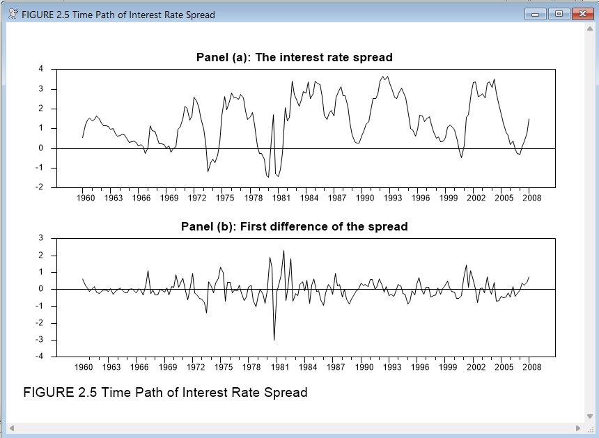
Next, we need to compute the interest rate spread. We will also want to examine the first differences of the series, so we will go ahead and compute those as well, and then graph both series. We will use the SPGRAPH instruction to display two graphs on a single page:
set spread = r10 - tbill
diff spread / dspread
spgraph(vfields=2,$
footer="FIGURE 2.5 Time Path of Interest Rate Spread")
graph(header="Panel (a): The interest rate spread")
# spread
graph(header="Panel (b): First difference of the spread")
# dspread
spgraph(done)
Looking at the first panel, we don’t see strong evidence of a trend or any structural breaks, and the overall behavior suggests that the series is covariance-stationary. The first differences on the other hand (in panel b), behave much more erratically. Based just on looking at the data, it appears that we will want to model the series in levels, rather than in differences.
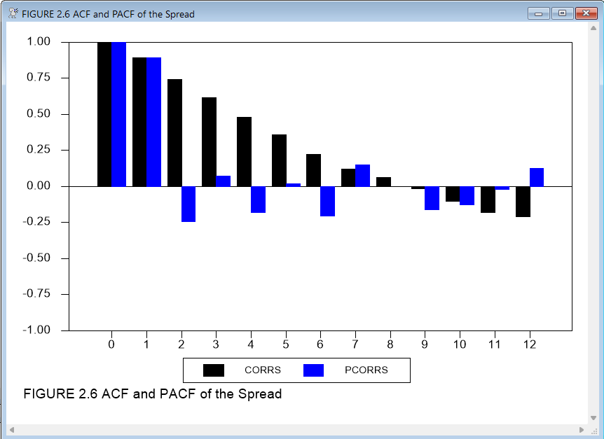
We can now examine the autocorrelation behavior of the series to identify some candidate models. The easiest way to do this is with the procedure @BJIDENT. First, we’ll show here how to generate the required graphs directly. We use the instruction CORRELATE to compute the statistics (autocorrelations and partial autocorrelations). The example below shows the options that we like to use for graphing these. Note that this graph includes the 0 lag statistics, which are always 1.0. At this stage of the modeling process (called the identification phase by Box and Jenkins), we find it helpful to leave this in as a reference. We’ll take it out in a later stage, when we’re expecting the autocorrelations at positive lags to be near zero.
corr(results=corrs,partial=pcorrs,number=12) spread
graph(header="Correlations of the spread",key=below,$
style=bar,nodates,min=-1.0,max=1.0,number=0) 2
# corrs
# pcorrs
As a further check on whether differencing the series is appropriate, we can examine the correlations of the first difference:
corr(results=dcorrs,partial=dpcorrs,number=12) dspread
graph(key=below,style=bar,nodates,min=-1.0,max=1.0,number=0, $
header="Correlations of the first difference of spread",) 2
# dcorrs
# dpcorrs
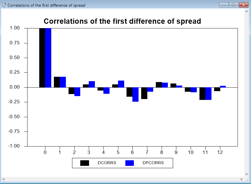
This series could go either way—the first difference series shows only mild signs of overdifferencing (correlations switching signs). Since you should take the minimal level of differencing to produce stationarity, we’ll stick with the undifferenced data.
A Note on Differencing
For models that do require differencing, you can either estimate the model using the differenced dependent variable, or you can use the original dependent variable and add a DIFFS option to include the differencing as part of the instruction. This has no effect on the estimates, and the only change in the output will be in the \(R^2\) and related measures. There are two advantages to having BOXJENK do the differencing:
1.It allows comparable \(R^2\) for models with different choices for the number of differences. Note, however, that the \(R^2\) is not considered to be an important summary statistic in ARIMA modeling.
2.If you define a forecasting equation using BOXJENK, it will be for the variable of interest, and not for its difference.
Selecting and Estimating Models
Our next step is to examine the autocorrelations and partial autocorrelations of the levels to identify some possible models. We can see that the autocorrelation functions decay fairly slowly, rather than either cutting off immediately (as they would for a pure MA process) or decaying geometrically (as they would for an AR(1) process). This suggests that we will need a higher-order AR model, or a model including both AR and MA terms.
As Enders explains in his text, the fact that there are significant partial autocorrelation values as far out as seven lags suggests that we may need AR terms out to six or seven lags. Also, the pattern of alternating positive and negative partial autocorrelations suggest the presence of a (positive) MA term, as well as one or more AR terms.
Enders starts by estimating six possible models. We will include the code for three of them here—see ARIMA.RPF for the others. First, though, some
general points on estimating and comparing ARIMA models using the BOXJENK instruction.
RATS offers two criterion functions for fitting ARMA models: conditional least squares and maximum likelihood. The default is conditional least squares—use the MAXL option on BOXJENK to get maximum likelihood instead. Each method has its advantages. Conditional least squares has a better behaved objective function, and thus is less likely to require “fine tuning” of the initial guess values. However, there are several ways to handle the pre-sample values for any moving average terms, so different software packages will generally produce different results. Maximum likelihood is able to use the same sample range for all candidate models sharing the same set of differencings, and so makes it easier to compare those models. The RATS procedure @BJAUTOFIT uses maximum likelihood for precisely this reason. In addition, maximum likelihood estimates should give the same results across software packages.
The most interesting summary statistics in the BOXJENK output are the standard error of estimate (for conditional least squares) or the likelihood function (for maximum likelihood) as your measure of fit, and also the \(Q\) statistic. Ideally, you would like the \(Q\) to be statistically insignificant. In addition, it’s standard practice to examine the autocorrelations of the residuals, looking for large individual correlations. The \(Q\) can pick up general problems with remaining serial correlation, but isn’t as powerful at detecting a few larger-than-expected lags. For residuals, it generally makes more sense to do the autocorrelations only (not partials).
Our model is going to include an intercept, as we expect a non-zero mean. There are three main ways that software packages deal with the intercept:
a.Remove the mean from the differenced data, then add it back after estimating the model on the mean zero data.
b.Include the intercept as a coefficient in a “reduced form” model.
c.Separate the model into a “mean model” and a “noise model”.
RATS normally uses (c). (You can implement the first using the option DEMEAN). For an AR(1) model, the difference between (b) and (c) is that (b) estimates the model in the form \(y_t = c + \phi y_{t - 1} \), while (c) does \(y_t - \alpha = \phi (y_{t - 1} - \alpha )\). The two models should produce identical answers (with \(c = \alpha (1 - \phi )\)) given the same method of estimation.
The advantages of the form chosen by RATS is that the estimated coefficient on the constant has a simple interpretation as the mean of the differenced process. It also generalizes better to intervention models and the like.
In this case, we estimate the candidate models by unconditional least squares. To ensure comparability, they are all run over the same sample range, from 1961:4 to the end of data. 1961:4 is the earliest period for which the model with the longest lag length—the AR(7) model—can be run using conditional least squares.
The estimates in the Enders text use method (b) to handle the mean. As you can see, all other results are unaffected by this choice.
An AR(7) Model
The instruction below estimates our first model, an AR(7) with a constant term:
boxjenk(constant,ar=7) spread 1961:4 *
This reports the \(Q\) for 36 lags as 28.71 with 29 degrees of freedom, which is not significant, showing no evidence of residual serial correlation. Note that the output shows 36–7 for the degrees of freedom: the number of autocorrelations used (36) minus the number of estimated ARMA parameters.
Q(36-7) 28.7150
Significance Level of Q 0.4799810
Next we compute and graph the residual autocorrelations and some additional \(Q\) statistics. We use the DFC option on CORRELATE to correct for the degrees of freedom used in the estimation, which will be the number of AR and MA parameters. BOXJENK saves that value for us in the %NARMA variable. The NUMBER and SPAN options tell RATS to compute correlations out to 12 lags and to report \(Q\) statistics for every 4 lags. (We’ll show you an easier way to do this in a moment).
correlate(results=rescorrs,number=12,span=4,qstats,$
dfc=%narma) %resids
graph(header="AR(7)",style=bar,nodates,min=-1.0,max=1.0,number=1)
# rescorrs 2 *
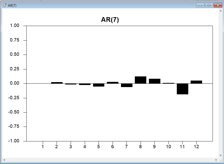
The autocorrelation plot offers further evidence that there is little remaining correlation in the residuals. These are the \(Q\) statistics for lags 4, 8, and 12 produced by CORRELATE:
Ljung-Box Q-Statistics
Lags Statistic Signif Lvl
4 0.230
8 4.501 0.033868
12 13.072 0.022714
While these are apparently significant, that is mainly because we have very few degrees of freedom after correcting for the seven estimated ARMA parameters. You can see from the graph why you need to correct for the number of estimated parameters, since the AR(7) model almost completely eliminates autocorrelation for 1 to 7.
While the model seems adequate, we don’t yet know if it does a good job of forecasting the data, or whether other models might do a better job. The rather large number of parameters suggests there might be a smaller model which will do better.
The @REGCORRS Procedure
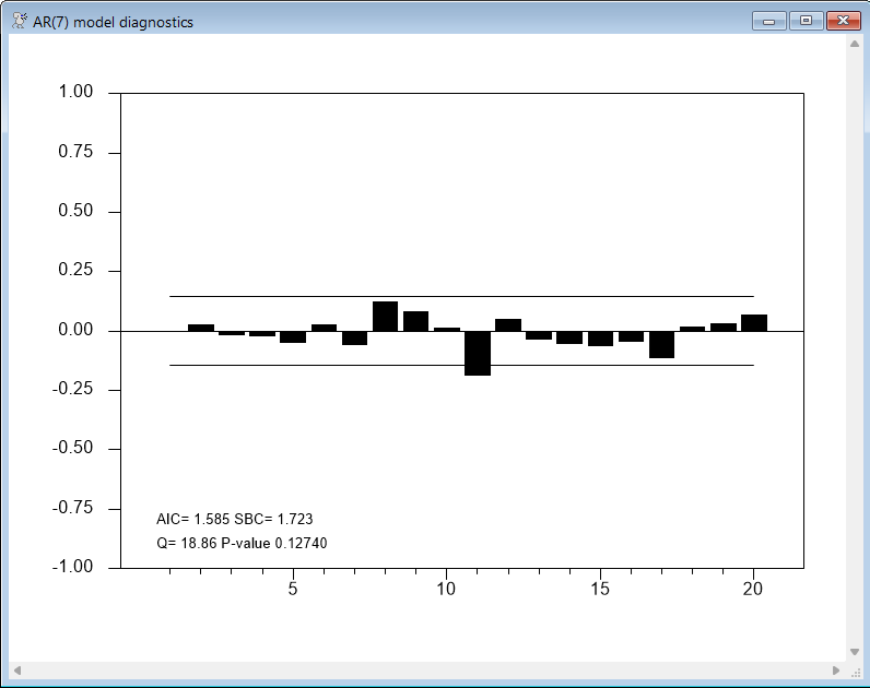
Although it is useful to know how to compute and graph the correlations using the CORRELATE and GRAPH instructions, in practice you will probably prefer to use the @REGCORRS procedure. @REGCORRS displays standard error bands on the correlation plots, Akaike (AIC) and Schwarz Bayesian (SBC) information criteria statistics, and (with the REPORT option) produces a table of \(Q\) statistics for the residuals from the most recent estimation (which are automatically stored in %RESIDS). We’ll describe the procedure in more detail later, but for now, here’s a simple example:
boxjenk(constant,ar=7) spread 1961:4 *
@regcorrs(dfc=%narma,number=20,qstats,report,$
method=burg,title="AR(7) model diagnostics")
Other Candidate Models
Given that models with fewer parameters often forecast as well as, or better than, larger models, we will look at two of the smaller models Enders considers—an AR(2) model and an ARMA(1,1):
boxjenk(constant,ar=2) spread 1961:4 2008:1
@regcorrs(dfc=%narma,number=20,qstats,report,$
method=burg,title="AR(2) model diagnostics")
boxjenk(constant,ar=1,ma=1) spread 1961:4 2008:1
@regcorrs(dfc=%narma,number=20,qstats,report,$
method=burg,title="ARMA(1,1) model diagnostics")
In both cases, the \(Q\) statistics and correlation plots suggest the presence of significant correlations in the residuals. For example, here are the results for the AR(2) model:
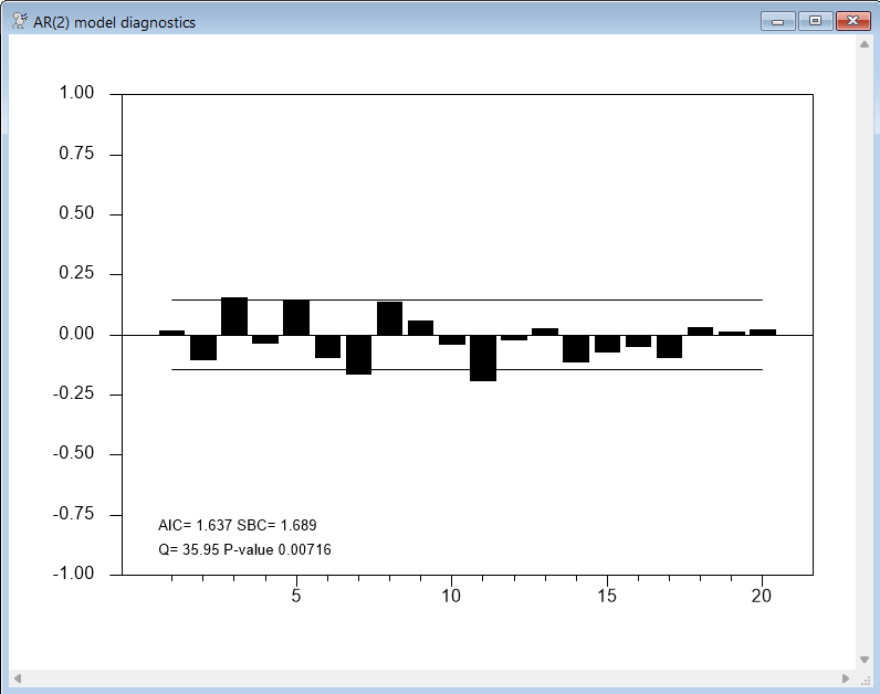
So, these particular models are not accounting for all of the correlation behavior, and are unlikely to provide reliable forecasts.
Enders finds that an ARMA(2,1) model performs better than the ARMA(1,1) model, but leaves some significant correlations around lag 7, and so he next considers a model with AR terms at lags 1 and 2, and MA terms on lags 1 and 7. This kind of model is handled easily in RATS, by using the in-line matrix notation (||value,value,...,value||) to provide a list of lags:
boxjenk(constant,ar=2,ma=||1,7||) spread 1961:4 2008:1
@regcorrs(dfc=%narma,number=20,qstats,report,$
method=burg,title="ARMA(2,(1,7)) model diagnostics")
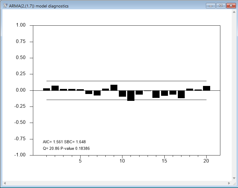
Both the AR(7) and ARMA(2,(1,7)) models look promising. The AIC criteria (computed by @REGCORRS) favors the AR(7) model, while the SBC criteria favors the ARMA(2,(1,7)).
The next step is to compare the forecasting performance of these two models. To do this, we need to include the DEFINE option on the BOXJENK instructions that estimate the model. We can then use the instruction UFORECAST to compute the forecasts.
First, we’ll estimate both models through 1995:3, holding back the last fifty observations of data. We then compute forecasts for those fifty periods, and generate a graph comparing the forecasts with the actual values. Note, by the way, that these are multiple step dynamic forecasts.
boxjenk(constant,define=ar7eq,ar=7) spread * 1995:3
boxjenk(constant,define=ar2ma17eq,ar=2,ma=||1,7||) spread * 1995:3
uforecast(equation=ar7eq,print) fore_ar7 1995:4 2008:1
uforecast(equation=ar2ma17eq,print) fore_ar2ma17 1995:4 2008:1
graph(header="Forecasts vs Actuals",key=upleft) 3
# spread 1995:1 *
# fore_ar7
# fore_ar2ma17 / 5
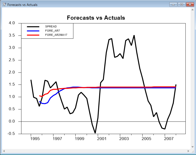
The results are rather typical of time series forecasts for models that do not include a trend: after the two years or so, the forecast is almost a straight line. As mentioned earlier, the long-term forecasts are dominated by the choice of differencing (if any) plus the intercept. Here, with no differencing applied, both forecasts eventually (in this case after about two years) level out at a constant value.
Now, we’ll look at how well the models fare when forecasting just one step beyond the end of the estimation range. Naturally, the one-step forecasts track much better than the multi-step forecasts. This code loops over our 50 periods of holdback data, estimating through entry T–1 and forecasting entry T, for T=1995:4 through 2008:1.
do time=1995:4,2008:1
* Estimate through period TIME-1
boxjenk(noprint,constant,define=ar7eq,ar=7) spread * time-1
boxjenk(noprint,constant,define=ar2ma17eq,ar=2,ma=||1,7||) $
spread * time-1
* Forecast one step ahead (entry TIME)
uforecast(equation=ar7eq,static) forecast_ar7 time time
uforecast(equation=ar2ma17eq,static) forecast_ar2ma17 time time
end do
* Graph the forecast with the actuals.
graph(header="Forecasts vs Actuals",key=upleft) 3
# spread 1995:1 *
# forecast_ar7
# forecast_ar2ma17eq / 5
Forecast Errors and Theil U Statistics
For one-step ahead forecasts, we can use the @UFOREERRORS procedure to quickly compute forecast performance statistics:
@uforeerrors spread forecast_ar7
@uforeerrors spread forecast_ar2ma17
To look at forecast performance over longer horizons, we can use the instruction THEIL. This does a series of multiple step forecasts and does parallel analysis on each horizon. One of the statistics that it computes is Theil’s U statistic. This is the ratio between the RMS errors of the model’s forecasts to the RMS errors of a “naive” forecast of no change in the dependent variable from the previous value. See the description of THEIL for details. This has the advantage over the basic error statistics like the RMSE as it is scale-independent, and also offers a quick comparison with another forecasting procedure. Here’s how to use this for our ARMA model. We compute forecasts for (up to) 8 steps ahead for each starting date in the range 1995:4 through 2008:1. The model is re-estimated after each set of forecasts to use the next available data point.
boxjenk(constant,define=ar2ma17eq,ar=2,ma=||1,7||) spread * 1995:3
theil(setup,steps=8,to=2008:1)
# ar7eq
do time=1995:4,2008:1
theil time
boxjenk(noprint,constant,define=ar2ma17eq,ar=2,ma=||1,7||) $
spread * time
end do time
theil(dump,title="Theil U results for ARMA(2,(1,7)) Model")
The results are as follows:
Theil U results for ARMA(2,(1,7)) Model
Step Mean Error Mean Abs Err RMS Error Theil U N Obs
Forecast Statistics for Series SPREAD
1 0.0131677 0.3449180 0.4389769 0.9477 50
2 0.0221656 0.5791501 0.7038170 0.9279 49
3 0.0155860 0.7343455 0.8825325 0.8821 48
4 -0.0035745 0.8302931 1.0263826 0.8485 47
5 -0.0270086 0.9029884 1.1094199 0.8158 46
6 -0.0347677 0.9691531 1.1482820 0.7892 45
7 -0.0416368 0.9942000 1.1574798 0.7613 44
8 -0.0474994 1.0144249 1.1664960 0.7320 43
These results are slightly superior (smaller errors and Theil U’s at each horizon) than the results for the AR(7) model, but the differences between the two sets of results are small. Overall, they suggest that both models should provide adequate (and comparable) forecasts.
We will now show how to use specialized procedures to do many of these tasks.
The procedure @BJTRANS can help you determine the appropriate preliminary transformation if you are unsure which to use. It graphs the series, its square root and its log on a single graph so you can compare their behavior. You are looking for a transformation which “straightens” out the trend (if there is one), and produces approximately uniform variability. The graph also shows a (very crude) log likelihood of a model under the three transformations. You shouldn’t necessarily choose the transformation based upon which of these is highest, as a close decision might be reversed with a careful model for the transformed processes. However, if there is a very clear difference among the likelihoods, they are likely to be pointing you to the best choice. The syntax is:
@bjtrans series start end
We can’t apply @BJTRANS to the SPREAD series, as it contains non-positive values (so the square root and log transforms won’t work). To demonstrate how this works, we can apply the procedure to a producer price index series that is also included on the QUARTERLY.XLS file:
data(format=xls,org=columns) / ppinsa
@bjtrans ppinsa
Now, this is a series which we expect to be best modeled in logs, and the log likelihood values would support that. The levels (“None”) are clearly inadequate. Note, from the graph, that there is effectively no visible short-term movements in the first half of the sample, while it is considerably less smooth in the second half, but the log transform gives a more uniform variability across the full sample.
![]()
@BJDIFF can aid in choosing the proper set of differences for a series. It generates a table of BIC criteria for various combinations of differencings and mean extractions. With non-seasonal data the choice of differencing is usually either quite clear or doesn’t matter much. There are more options with seasonal data and the choice isn’t quite as obvious. In addition, the usual Box-Jenkins methodology uses a graphical procedure (helped by the @BJIDENT procedure) which won’t help if you need an automated process.
@bjdiff( options ) series start end
The main options are:
diff=maximum regular differencings[0]
sdiffs=maximum seasonal differencings[0]
span=seasonal span [CALENDAR seasonal]
trans=[none]/log/root
Chooses the transformation to apply to series.
@BJDIFF produces a table with a list of the possible combinations with the minimum BIC choice starred. It also defines %%AUTOD as the recommended number of regular differencings, %%AUTODS as the recommended number of seasonal differencings and %%AUTOCONST as the recommended choice for CONST option.
This is what we get from the SPREAD series. Above, we chose (in a close decision), no differences with a constant. @BJDIFF picks the alternative of 1 difference without the constant.
@bjdiff(diffs=1) spread
BJDiff Table, Series SPREAD
Reg Diff Seas Diff Intercept Crit
0 0 No -0.631763
0 0 Yes -0.879370
1 0 No -1.177689*
1 0 Yes -1.150394
The procedure @BJIDENT assists in identifying a Box-Jenkins model by computing and graphing the correlations of the series in various differencing combinations. Here is the syntax for the @BJIDENT procedure, with the most common set of options:
@bjident( options ) series start end
The range (start and end) default to the maximum usable range given the selected DIFFS/SDIFFS. (All analysis is done with a common range).
The main options set the maximum number of differencings: DIFFS=maximum regular differencings, SDIFFS=maximum seasonal differencings.
@BJIDENT examines every combination of regular and seasonal differencing between 0 and the maximums indicated. For instance, with each set at 1, it will do \(0 \times 0\), \(0 \times 1\), \(1 \times 0\) and \(1 \times 1\).
The option trans=[none]/log/root selects the preliminary transformation, though typically you will already have transformed the data in a separate step.
If you use the REPORT option, @BJIDENT will create a table of the computed statistics for the various differencing combinations. If you include QSTATS as well, it will compute Ljung-Box Q statistics and their significance levels. While some software does the Q statistics as part of their “ident” functions, we recommend against it. The Q’s are tests for white noise; they have no real implications for stationarity decisions, and at this point, we don’t expect to see the correlations pass a white noise test even with the correct number of differencings.
Examples
Recall the fairly complicated DIFF, CORR and GRAPH instructions that we used earlier to produce graphs of the correlations for both SPREAD and the first difference of SPREAD. Using @BJIDENT, the following is all you need to produce even fancier versions of these graphs:
open data quarterly.xls
calendar(q) 1960:1
data(format=xls,org=columns) / tbill r10 ppinsa
set spread = r10 - tbill
@bjident(diffs=1) spread
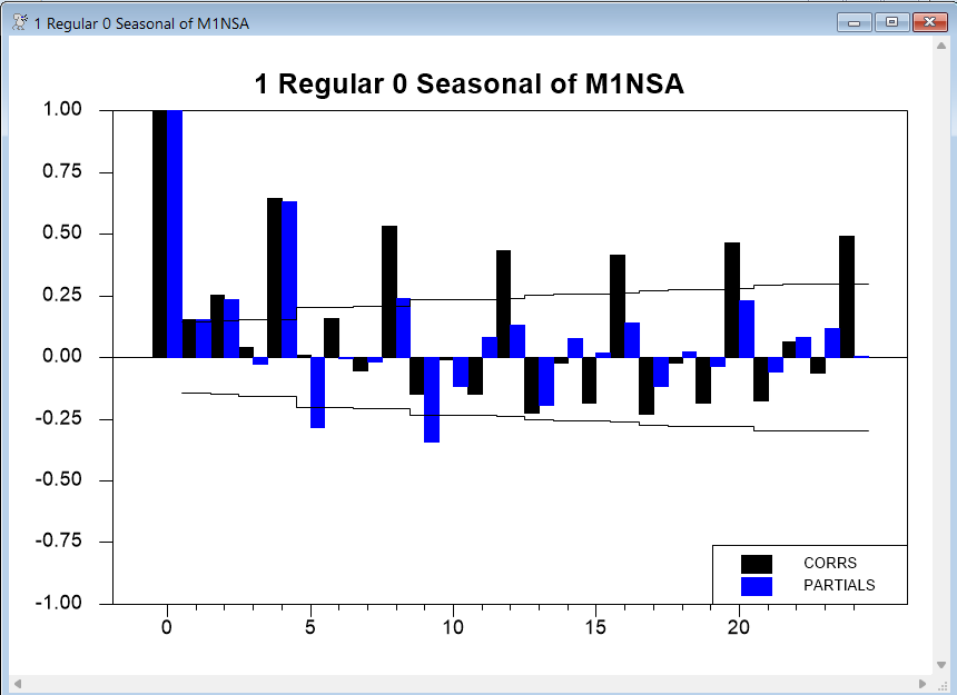
The next example produces graphs for all combinations of 0 or 1 regular difference and 0 or 1 seasonal differences for the log of M1NSA (a non-seasonal adjusted series of the U.S. M1 money supply (also available on QUARTERLY.XLS and discussed in Section 2.11 of the Enders text). It shows 24 correlations. We also include the REPORT and QSTATS options, to generate a report window containing the correlations and Q statistics at each horizon:
data(format=xls,org=columns) / tbill r10 ppinsa m1nsa
@bjident(diffs=1,sdiffs=1,trans=log,number=24,report) m1nsa
The graphs with no differencing make it clear that we need at least one regular difference. The graph with one regular difference but no seasonal difference suggests that we do in fact need a seasonal difference to deal with the persistent seasonality:
As you can see from the next graph, adding a seasonal difference accounts for most of the remaining correlation, but still does not account for all of the seasonality:
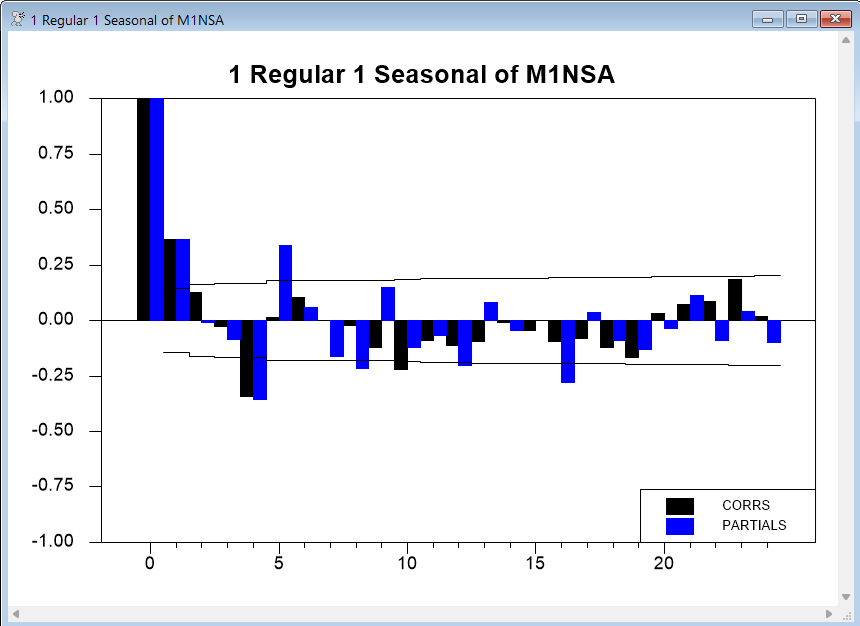
Enders settles on a model with AR(1) and SMA(1) (seasonal moving average) terms for these data.
The @BJFORE procedure provides an easy way to estimate and forecast an ARIMA model with a single instruction. The syntax is as follows:
@bjfore(options) series fstart fend forecasts
fstart and fend give the range to forecast. (The estimation uses all available information through fstart-1 unless you use the RSTART and REND options to override that.)
The options describe the model you are using (basically pass-throughs to the BOXJENK instruction) such as DIFFS, ARS and MAS.
Examples
Returning to our SPREAD example, we can estimate the model through 1995:3 and generate dynamic forecasts for 1995:4 through 2008:1 using just this line:
@bjfore(ars=7,constant) spread 1995:4 2008:1 fore
For our model for M1NSA, we can estimate the model and graph the results using the following:
@bjfore(ars=1,smas=1,trans=log,diffs=1,sdiffs=1,constant) m1nsa $
2008:2+1 2008:2+12 m1fore
graph(header="M1NSA: Actuals and Out of Sample Forecasts") 2
# m1nsa 2000:1 *
# m1fore
We introduced the @REGCORRS procedure earlier in this section. Recall that it computes and optionally graphs the residual autocorrelations, computing the \(Q\)-statistic and the AIC and SBC. It can be used after any type of single-equation estimation, not just after BOXJENK.
@regcorrs( options ) resids
Main Options
number=number of autocorrelations to compute [25 if possible]
dfc=degrees of freedom correction for Q statistics
[graph]/nograph
print/[noprint]
[qstats]/noqstats
report/[noreport]
[criteria]/nocriteria
title="title for report window"
header="graph header string"
footer="graph footer string"
If GRAPH, @REGCORRS creates high-resolution graphs of the correlations. If PRINT, the output from CORRELATE is included in the output window, and, if, in addition, you use QSTATS, that output will include the Q-statistics. If REPORT, a separate table is displayed with the correlations, partial autocorrelations and Q-statistics for different lag lengths.
NUMBER sets the number of autocorrelations to compute and graph. DFC should be set to the number of ARMA parameters estimated; BOXJENK sets the variable %NARMA equal to this.
In addition to the Q-statistic variables (%QSTAT, %QSIGNIF and %NDFQ), @REGCORRS also computes %AIC and %SBC, which are the Akaike Information Criterion and the Schwarz Bayesian Criterion. The values of these will also be displayed on the graph.
The @BJAUTOFIT procedure estimates (by maximum likelihood) all combinations of ARMA terms in a given range, displaying a table with the values of a chosen information criterion, with the minimizing model having its value highlighted with a *. Note that this can take quite a while to complete if the PMAX and QMAX are large. Also, some of the more complicated models may not be well-estimated with just a simple use of BOXJENK(MAXL). However, these estimation problems generally arise because of poorly identified parameters, which means that a simpler model would fit almost as well and would thus be preferred anyway. The syntax is as follows:
@BJAutoFit( options ) series start end
The range (start to end) defaults to the largest range possible given the data and any differences. The main options are PMAX=maximum number of AR lags to consider and QMAX=maximum number of MA lags to consider. The CRIT option decides which information criterion to use: the choices are AIC, BIC or SBC where the last two are synonyms. The DIFFS, SDIFFS and CONST options indicate your choices for level of differencing and inclusion of the constant.
Example
We use @BJAUTOFIT on the SPREAD data, looking at models up to an ARMA(7,7).
@bjautofit(constant,pmax=7,qmax=7,crit=sbc) spread
Here, the procedure selects the ARMA(2,1) model (as indicated by the *), which was one of our leading candidates earlier:
BIC analysis of models for series SPREAD
MA
AR 0 1 2 3 4 5 6 7
0 618.96 436.75 383.69 343.23 340.28 334.86 314.74 319.97
1 323.03 313.41 316.03 316.71 321.36 325.10 319.98 324.66
2 316.51 313.37* 322.32 320.41 324.12 329.98 363.25 335.19
3 320.84 318.49 321.27 324.01 329.26 333.43 335.75 336.20
4 319.63 324.70 321.66 329.10 326.68 329.63 330.91 333.26
5 324.83 326.19 327.67 326.34 325.85 336.49 334.75 335.70
6 321.86 324.50 322.75 333.07 339.78 333.38 347.77 466.51
7 322.89 327.09 329.74 338.85 338.12 346.98 359.14 489.79
The procedure does not allow for models with skipped lags, so it’s not surprising that it selects a slightly simpler model than the ARMA(2,(1,7)) we chose after noting some remaining correlation around lag 7 in the ARMA(2,1) residuals. This demonstrates that criterion-based selection tools can be helpful for narrowing down choices or verifying conclusions, but are no substitute for careful analysis and judgment.
The procedure saves the selected AR and MA values in the variables %%AUTOP and %%AUTOQ, so you can estimate the model and analyze the residuals by doing:
boxjenk(constant,define=ar2ma1eq,ar=%%autop,ma=%%autoq) spread
@regcorrs(dfc=%narma)
@GMAUTOFIT is similar to @BJAUTOFIT but is designed to choose the more complicated multiplicative seasonal ARMA model to a series. This follows the procedure described in Gomez and Maravall(2001). Because there are four polynomial lengths to choose and seasonal models take much longer to estimate than non-seasonal models, Gomez-Maravall searches for an approximate minimum BIC model. Rather than attempt an exhaustive search across all four simultaneously (though you can do that with the FULL option), it first fixes the “regular” ARMA parameters, then does an exhaustive search over the seasonal parameters only. Once those are chosen, they are fixed and an exhaustive search is done for the regular ARMA parameters. An example of its use is provided by AUTOBOX.RPF.
Copyright © 2026 Thomas A. Doan