Now we’ll look at an example to demonstrate some time series filtering and analysis techniques, and explore the graphing capabilities of RATS. It uses (non-seasonally adjusted) monthly data on housing starts in the United States, and is also from Pindyck and Rubinfeld (1998), page 480. The instructions are provided on the file ExampleFour.rpf. Before starting, close the Input Window and start a new one (with File—New—Editor/Text Window). This time, we will use separate input and output windows. Once the editor window is open, hit the  toolbar button.

 

The data file we want is called EX152.XLS. Use the Data/Graphics—Data Wizard (Other Formats) operation to open the file. Click on “Scan” to process the date information. The dialog box should look like this:

 

 

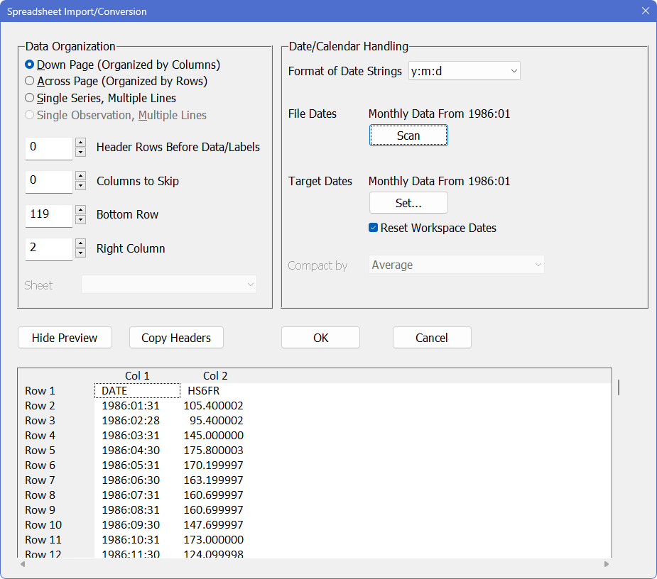
The dates are in the form “year:month:day”, but the file only contains one observation per month. RATS is able to recognize this, and correctly identifies this as monthly data. Click on “OK”. RATS will generate and execute (something like: the location of the file will be different) the following instructions:

 

OPEN DATA "C:\RATS\ex152.xls"

CALENDAR(M) 1986:1

DATA(FORMAT=XLS,ORG=COLUMNS) 1986:01 1995:10 HS6FR

Examine the Data

As always, we recommend that you examine the data before proceeding. For example, select View—Series Window from the menu, click on the HS6FR series, and do View–Time Series Graph. You should see the following:

 

 

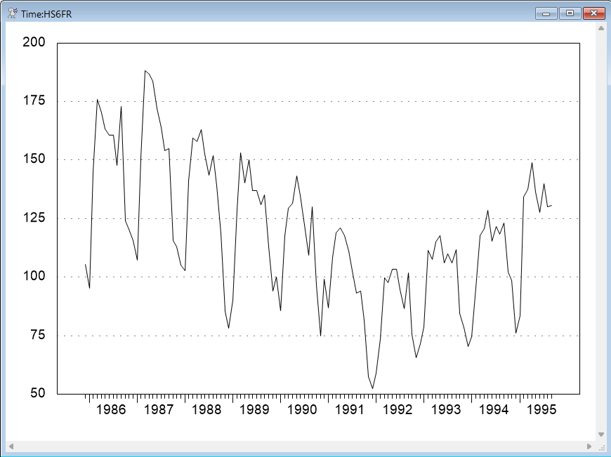
As you would expect, the series exhibits a very strong seasonal behavior. There also appears to be a decreasing trend over the first few years, followed by an increasing trend over the remaining years.

Filtering and Smoothing

We will examine some techniques for smoothing the data. Start by selecting Data/Graphics—Filter/Smooth, which will bring up this dialog box:

 

 

Because we only have one series in memory (HS6FR), RATS automatically selects it as the “Input Series”. The default filter type is a centered flat moving average filter, which is what we want (“centered” means that for a window width of \(2N+1\) periods, the filtered value at time \(T\) is computed using observations \(T-N\) through \(T+N\)).

 

Type in FLAT7 as the name for the “Output Series”, and enter 7 as the “Width”:

 

 

Click on “OK”. RATS will generate a FILTER instruction with the appropriate options:

 

FILTER(TYPE=CENTERED,WIDTH=7) HS6FR / FLAT7

 

This seven-period moving average should smooth the series considerably, but will probably retain some of the seasonal behavior. To reveal the underlying trend behavior of this series, we can try the Hodrick-Prescott (HP) filter. It is designed to separate the trend behavior of a series from its cyclical component. Select Data/Graphics—Filter/Smooth again. This time, you’ll have to select HS6FR as the input series (RATS doesn’t guess, now that there is more than one series in memory). Enter HPFILTER as the “Output Series” and select “Hodrick-Prescott” as the “Filter Type”. You can leave the "Tuning" parameter field blank to use the default value. The dialog should look like this:

 

 

Click "OK" and this will generate:

 

FILTER(TYPE=HP) HS6FR / HPFILTER

Graphing the Data

Let’s examine the results by generating a graph that includes all three series. This time we will use the Data/Graphics—Graph operation on the menu. Unlike View–Time Series Graph, this actually generates a RATS instruction, making it easy to reproduce the graph later. It also gives us more control over the appearance of the graph.

 

Select the Data/Graphics—Graph operation, which displays this dialog box:

 

 

 

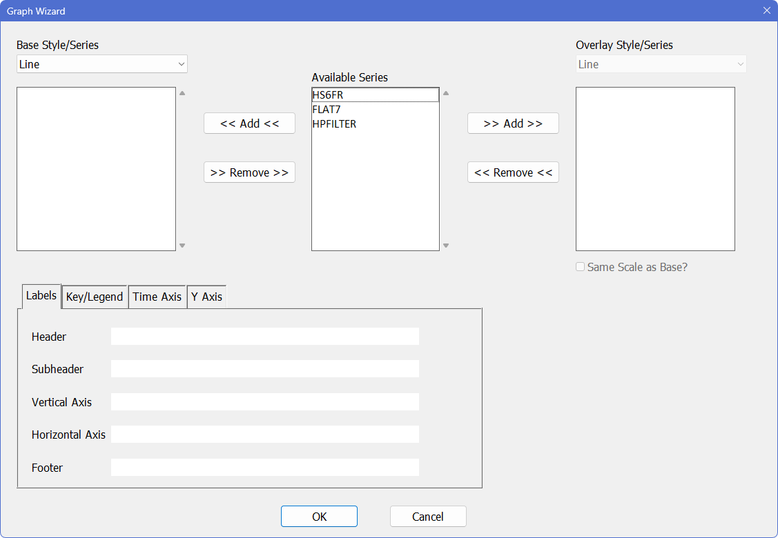
The “Series” field in the middle lists all the series available in memory. We want to graph all three, so click on HS6FR and then <Shift>+click on HPFILTER to highlight the whole list. Click on the  button to add the three series to the “Base Series” list on the left (as opposed to the “Overlay Series” list on the right, which is used to graph some series using a second vertical scale).

 

That’s all you need to do to produce a graph, but let’s add some features. First, type in “Moving Average versus HP Filtering” in the “Footer” field at the bottom. The dialog should now look like this:

 

 

Next, click on the “Key/Legend” tab, and select “Upper Right (Inside)” as the position for the key. Then click “OK” to generate the graph.

Here’s the resulting Graph Window:

 

 

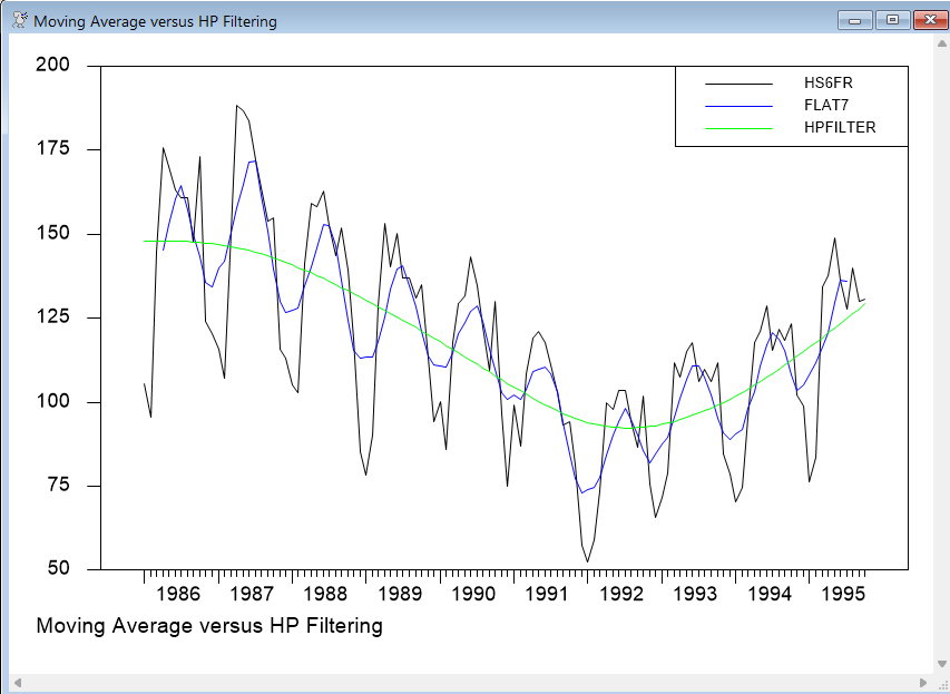
As expected, FLAT7 is considerably smoother than the original series, but still shows a significant amount of seasonality. The HPFILTER series, however, seems to fit the overall trend behavior of the original series quite well, with nearly all of the cyclical behavior and short-term fluctuations removed.

 

Here is the GRAPH instruction generated by the wizard:

 

GRAPH(STYLE=LINE,FOOTER="Moving Average versus HP Filtering",KEY=UPRIGHT) 3

# HS6FR

# FLAT7

# HPFILTER

 

The main instruction includes several options: STYLE, which controls the way data is represented;  FOOTER, which adds a text label below the graph; and KEY, which adds a key. Both STYLE and KEY select from a specific list of choices—see the description of GRAPH for a list of the possible choices. The number “3” at the end of the GRAPH line tells RATS that you are graphing three series.

 

When you are done viewing the graph, close the graph window or click on the input window to bring it back to the front.

Detrending, Exponential Smoothing, Forecasting

Pindyck and Rubinfeld also examine the use of exponential smoothing techniques. First, they remove the trend component from the series by regressing it on a linear trend series. Then they apply exponential smoothing to get a smoothed version of the detrended series. They then add back the trend component removed in the first step to get a smoothed version of the original series.

 

This can actually be done in a single step in RATS. We’ll demonstrate that in a moment, First, here is the step-by-step version.

 

The Filter/Smooth operation offers one way of removing a trend using a regression. Select Data/Graphics—Filter/Smooth, and choose HS6FR as the input series. Type in DETREND as the output series, select “OLS Trend/Seasonal Removal” as the filter type, and turn on the “Trend” checkbox:

 

 

Click “OK” to generate the DETREND series. The instruction looks like this:

 

FILTER(REMOVE=TREND) HS6FR / DETREND

 

Next, we need to compute and save the trend component that was removed, by subtracting the detrended series from the original series. You could use the Data/Graphics—Transformations wizard to do this, but you may find it easier just to type in the SET instruction yourself:

 

set removed = hs6fr - detrend

 

Now, we can do our exponential smoothing on the detrended series. Because it is time-series specific, the Exponential Smoothing wizard is located on the Time Series menu. Go ahead and select Time Series—Exponential Smoothing.

 

Select DETREND as the input series, “None” as the “Form for Trend”, and type in the name ESMOOTH for the "Smoothed Series". The textbook uses a value of 0.2 for the “level” smoothing parameter \(\alpha\), so enter that value in the “Level” field. The dialog box should look like this:

 

 

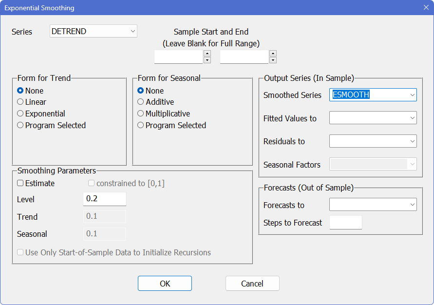
Click on “OK” to generate the ESMOOTH instruction:

 

ESMOOTH(ALPHA=0.2,SMOOTHED=ESMOOTH) DETREND

 

Now we need to add back in the trend component removed earlier. We can replace the existing values of ESMOOTH with the sum of those values and REMOVED:

 

set esmooth = esmooth+removed

 

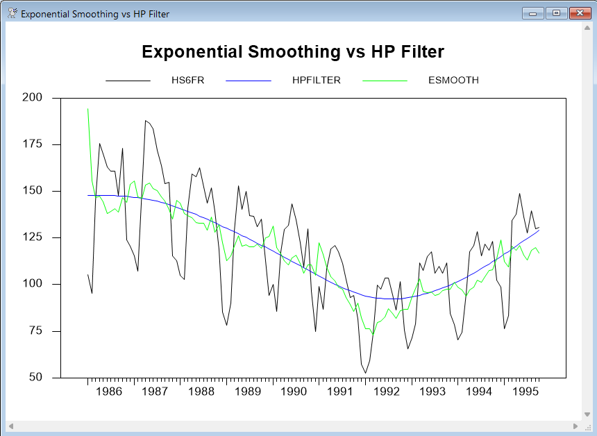
Now, select the Data/Graphics—Graph operation again, and choose HS6FR, HPFILTER, and ESMOOTH as the series to be graphed. To label the graph, enter “Exponential Smoothing vs HP Filter” as the header. On the "Key" tab, choose “Above (Outside)” and turn off the “Box Around Key?”:

 

 

This generates the instructions and graph shown below:

 

GRAPH(STYLE=LINE,HEADER="Exponential Smoothing vs HP Filter",KEY=ABOVE,NOKBOX) 3

# HS6FR

# HPFILTER

# ESMOOTH

 

 

Modelling the Trend and Seasonal Behavior

As noted earlier, there is an easier way to do this, which is to include a component for the trend behavior in the exponential smoothing model. Select Time Series—Exponential Smoothing again. This time, select the original series HS6FR as the series to model. Then, select the "Linear" choice for the trend model in the “Form for Trend” box, and turn on the “Estimate” switch in the “Smoothing Parameters” box (which tells RATS to estimate the smoothing parameters used in the model).

 

That’s all you need to reproduce the previous analysis, but let’s go a couple of steps further, by also including a seasonal term in the model and using the resulting model to produce forecasts.

 

In the “Form for Seasonal” box, select “Multiplicative”. Provide a name for the "Smoothed Series" (we used ESMOOTH again here). Finally, enter a name in the “Forecasts to” box to hold the forecasts (we use ESMOOTH_FORE), and enter 8 as the number of forecast steps to compute. The dialog should look like:

 

 

When you are ready, click “OK” to do the smoothing. The resulting instruction is shown below (we split the line for readability), along with a GRAPH instruction that plots both the original series and the forecasts.

 

ESMOOTH(TREND=LINEAR,SEASONAL=MULTIPLICATIVE,ESTIMATE,SMOOTHED=ESMOOTH,$

   FORECAST=ESMOOTH_FORE,STEPS=8) HS6FR

GRAPH(STYLE=LINE,HEADER="Exponential Smoothing Forecast",KEY=ABOVE,NOKBOX) 3

# HS6FR

# ESMOOTH

# ESMOOTH_FORE

Seasonally Adjusting Data

If you just want to seasonally adjust (de-seasonalize) the data, you would include a seasonal component in the ESMOOTH model, but omit the trend term. The ESMOOTH below does just that, and saves both the smoothed (seasonally adjusted) values and the fitted values. This also uses the ESTIMATE option to estimate the values of the model coefficients.

 

esmooth(seasonal=multiplicative,estimate,smoothed=smoothed,fitted=fitted) hs6fr

graph(header="Seasonally Adjusted Data",key=above,nokbox) 3

# hs6fr

# smoothed

# fitted

 

 

As you can see from the graph, the seasonal component has been removed from SMOOTHED, leaving the underlying trend and short-term fluctuations.

 

Exponential smoothing offers a relatively simple form of seasonal adjustment. You can also treat seasonality using state-space models or, if you have a Professional level of RATS, you can use the more sophisticated Census X11/X12 adjustment procedure.

Regression-based Forecasting

The graph shows general upward trend from 1992 on in the seasonally adjusted series. Suppose we want to generate an out-of-sample forecast of that trend through 1996. One way to do that is to do a simple regression on a constant and a trend series.

 

First, we need to define the trend series. Because we’ll be forecasting out-of-sample, we need to define that trend series beyond the end of the actual data to include the forecasting range (the special built-in CONSTANT series is automatically available at all time periods).

 

Select Data/Graphics—Trend/Seasonals/Dummies. Enter TREND as the series name, and 1996:12 as the ending date:

 

 

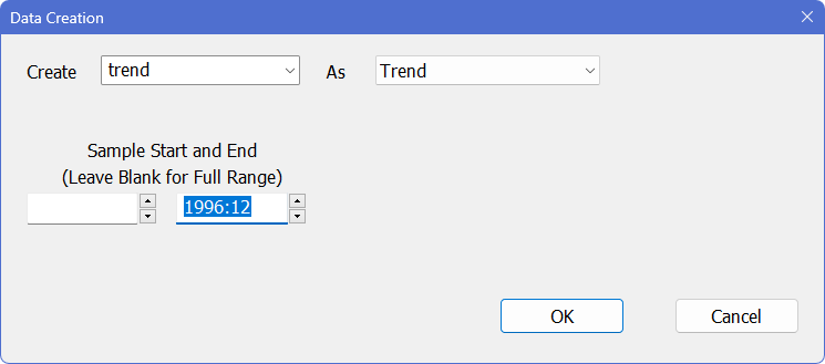
This generates the instruction:

 

SET TREND * 1996:12 = T

 

which uses the (normally omitted) start and end parameters on SET. The * symbol used for the start parameter tells RATS to use the earliest date in the default range (entry one in this case). Specifying 1996:12 as the end date defines the trend through the end of our forecast range.

 

The T on the right side of the equal sign is a reserved variable in RATS. It returns the current entry being set or evaluated. So, this creates a series called TREND that contains the number 1 in entry 1, the number 2 in entry 2, and so on.

 

Next, select Statistics—Linear Regressions, and enter SMOOTHED (the seasonally adjusted series) as the dependent variable, 1992:1 as the starting date, CONSTANT and TREND as the explanatory variables, and FORECAST_EQ in the "Define Equation" box. The dialog box should look like this:

 

 

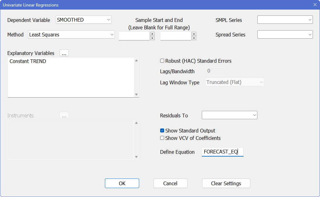
This generates the following LINREG:

 

LINREG(DEFINE=FORECAST_EQ) SMOOTHED

# Constant TREND

 

The DEFINE option creates an equation called FORECAST_EQ containing the structure and estimated coefficients from the regression. We’ll use that to produce forecasts.

 

Now select Time Series—Single-Equation Forecasts. The “Equation” field tells RATS which equation you want to forecast. The default choice (“Last Regression”) would actually work, because the last regression performed is the one we want to forecast, but go ahead and select FORECAST_EQ. Then, enter 1995:11 and 1996:12 as the starting and ending date for the forecasts. Finally, enter HSFORE in the “Forecasts To” field to save the computed forecasts into a series with this name:

 

 

Click “OK” to compute the forecast. This generates the following UFORECAST instruction (the U stands for univariate, or single-equation):

 

UFORECAST(FROM=1995:11,TO=1996:12,EQUATION=FORECAST_EQ) HSFORE

 

To see the results, execute the following—note the use of the date ranges to limit the graph to our estimation and forecasting range (we don’t need a range on HSFORE because it is only defined over the range we want to see):

 

graph 3

# hs6fr 1992:1 *

# smoothed 1992:1 *

# hsfore

Learn More: Graph Windows

Learn More: Long and Short Program Lines

Learn More: RATS Program Files (RPF)

 

At this point, you should have a complete Editor Window with the instructions for the analysis that we’ve done with this housing data series. The advantage of using the separate I/O windows is that we have the input commands by themselves. We will now save this as a RATS program file which we can run later.

 

Select File—Save (or File—Save As... or the  toolbar) and assign the file a name. For example, you might save this as MyProgram.rpf. You can also save the file when you close the window—you’ll be first asked if you want to save the changes, and if you answer “Yes”, you’ll be prompted for the file name.

 

 

Learn More: The PRINT Instruction

 

Another useful instruction for examining your data is PRINT. This displays series to the output window or (with a WINDOW option) to a spreadsheet-style window. If you want RATS to print all the data for all the series in memory, just type:

 

          print

 

To view data over a limited range of entries, you can add start and end parameters with the desired dates (or entry numbers):

 

print 1990:1 1996:6

 

You can also print only certain series by listing them after the dates:

 

print 1990:1 1996:6 hs6fr esmooth esmooth_fore

 

If you want all the data but only for certain series, you can replace the start and end parameters with a forward slash (/). This tells RATS to use the default range for the series:

 

print / hs6fr esmooth esmooth_fore

 

To display the information to a spreadsheet style window, add a WINDOW option and a title for the window:

 

          print(window="ESMOOTH Forecasts") / hs6fr esmooth_fore

 

You can copy and paste the contents of the resulting window into another program, or export the window contents to a spreadsheet or other file type using File–Export....

 

PRINT is also very useful when you are troubleshooting a program. When you get unexpected results, such as an error message complaining about missing values, try printing out the series involved. You may notice an error that had slipped through earlier checks.

 

You can use the PICTURE option to supply picture codes to control the formatting of the output. In this case, we use * on the left of the decimal, which tells RATS to use as many digits as necessary, while the .# tells RATS to round the output to one decimal.

 

print(picture="*.#") / hs6fr

 

  ENTRY         HS6FR

 1986:01        105.4

 1986:02         95.4

 1986:03        145.0

 1986:04        175.8

 

 

Learn More: Data Transformations

SET (introduced in Example Three) is the general data transformation instruction. RATS also has several special-purpose instructions for doing transformations, such as SEASONAL for creating seasonal dummies and DIFFERENCE and FILTER (above) for difference and quasi-difference transformations. However, most of the time you will be using SET. In "Data Transformations", we describe SET in more detail, and present a kit of standard data transformations. Most of those examples are not based upon the data sets we have been using, so you won’t necessarily be able to execute them as part of the tutorial. It should be easy to adapt them to your own needs, however.

 

 

Learn More: Forecasting

 

RATS can forecast using a wide range of modelling techniques:

•Simple regression models

•Vector autoregressions (VAR’s)

•Exponential smoothing

•Box-Jenkins (ARIMA) models

•Simultaneous equations

•State-Space Models

•Spectral methods

 

Forecasting Wizards and Instructions

You can use the PRJ instruction to compute out-of-sample fitted values for the most recently executed regression, as long as the necessary right-hand-side variables are defined for the required time periods.

 

We introduced the UFORECAST instruction and the Single-Equation Forecast Wizard above. The other, more general,  forecasting instruction is FORECAST. It can forecast one equation or many, and can also be used to forecast non-linear models. You can use the Time Series—VAR (Forecast/Analyze) operation to generate a FORECAST instruction once you’ve defined a proper model.

 

By default, both UFORECAST and FORECAST do dynamic forecasting. That is, when computing multi-step forecasts, they use the forecasted values from initial steps as the lagged dependent variable values in computing the later forecast steps. Both can also do static forecasting if you use the STATIC option. Static forecasting means that actual values are used for any lagged dependent variable terms in the model.

Equations and Formulas

Above, we introduced the idea of defining equations and using UFORECAST to compute forecasts using equations. FORECAST can also produce forecasts for a formula, or a set of formulas. Note the distinction between equations and formulas:

 

          

 

Copyright © 2025 Thomas A. Doan